| Issue |
Manufacturing Rev.
Volume 1, 2014
|
|
|---|---|---|
| Article Number | 21 | |
| Number of page(s) | 10 | |
| DOI | https://doi.org/10.1051/mfreview/2014020 | |
| Published online | 18 December 2014 | |
Research Article
An efficient genetic algorithm for a hybrid flow shop scheduling problem with time lags and sequence-dependent setup time
1
Department of Mathematic, Payame Noor University, Tehran, Iran
2
Department of Industrial Engineering, Bu-Ali Sina University, Hamedan, Iran
3
Department of Industrial Engineering, Birjand University of Technology, Birjand, Iran
* e-mail: This email address is being protected from spambots. You need JavaScript enabled to view it.
Received:
24
November
2013
Accepted:
23
November
2014
Abstract
In this paper, a hybrid flow shop scheduling problem with a new approach considering time lags and sequence-dependent setup time in realistic situations is presented. Since few works have been implemented in this field, the necessity of finding better solutions is a motivation to extend heuristic or meta-heuristic algorithms. This type of production system is found in industries such as food processing, chemical, textile, metallurgical, printed circuit board, and automobile manufacturing. A mixed integer linear programming (MILP) model is proposed to minimize the makespan. Since this problem is known as NP-Hard class, a meta-heuristic algorithm, named Genetic Algorithm (GA), and three heuristic algorithms (Johnson, SPTCH and Palmer) are proposed. Numerical experiments of different sizes are implemented to evaluate the performance of presented mathematical programming model and the designed GA in compare to heuristic algorithms and a benchmark algorithm. Computational results indicate that the designed GA can produce near optimal solutions in a short computational time for different size problems.
Key words: Hybrid flow shop / Scheduling / Sequence-dependent time lags / Sequence-dependent setup times / Genetic algorithm
© M. Farahmand-Mehr et al., Published by EDP Sciences, 2014
 This is an Open Access article distributed under the terms of the Creative Commons Attribution License (http://creativecommons.org/licenses/by/4.0), which permits unrestricted use, distribution, and reproduction in any medium, provided the original work is properly cited.
1. Introduction
Among the production scheduling systems, hybrid flow shops scheduling (HFS) problem is one of the most distinguishable environments demonstrating numerous applications in real industrial settings [16]. In HFS, we have a set of n jobs and a set of g production stages owning several identical machines operating in parallel. Some stages may have only one machine, but in order to qualify the plant to be called a hybrid flow shop, at least one of stages must have several parallel machines. However, each job is allowed to be processed at only one machine in each stage. In HFS, all n jobs follow the same operational order (processing route) and need to be processed at all g stages from stage 1 to stage g. The processing time of each job i at each stage t is fixed and known in advance. In all shop scheduling problems, one of the most commonly-used objectives is to discover a production sequence of the jobs on the machines such that a criterion or a set of selected criteria are optimized.
The scheduling problem that leads to the minimum makespan tends to be NP-hard in general, with very few notable exceptions, even when the machines at each stage are identical and there are no more than two machines in each stage. Therefore, it is not usually possible to solve the proposed models in a reasonable time when dealing with actual production planning problems [1].
The flow of jobs in the considered plant is unidirectional. Each operation of a job is processed only by one machine in each stage. Each stage may have several parallel identical machines. These machines can be identical, uniform, or unrelated.
Many restrictions to the previous assumptions can be enforced in manufacturing industries due to modeling system in a more realistic method, such as minimum or maximum time lags between two successive operations, setup times which are either sequence-dependent or not, limited buffer capacity between two successive stages. Time lags are defined as the time intervals which must exist between the completion time of the processing of one job at one stage and the beginning time of the processing of that job at the next stage.
In this paper, a hybrid flow shop scheduling problem with a new approach considering time lags and sequence-dependent setup time in realistic situations is presented. Since few works have been implemented in this field, the necessity of finding better solutions is a motivation to extend heuristic or meta-heuristic algorithms. This type of production system is found in industries such as food processing, chemical, textile, metallurgical, printed circuit board, and automobile manufacturing.
The rest of this paper is organized as follows. Section 2 provides a literature review on the hybrid flow shop scheduling. An integer linear programming model is formulated and illustrated by a numerical example in Section 3. Section 4 explains the heuristic methods and the designed GA for solving the proposed model. Section 5 gives a complete computational evaluation to compare the performance of the designed GA and the employed heuristics. Finally, some conclusions on this study are given in Section 6.
2. Literature review
In this section, we present the related literature review of studies addressing sequence-dependent setup times (SDST) or time lags in hybrid flow shop scheduling. Due to the numerous researches implemented in the literature of flow shop scheduling, we only focus on recent and most related studies.
While many papers have been written in the area of scheduling hybrid flow shop, many of them are restricted to special cases of two stages, specific configurations of machines at stages, and to simplify the problem, setups are seldom considered in the scheduling. For those ones addressing setups, the setup times are fixed and included in processing times. However, in most real world cases, the length of the setup time depends on both jobs, which is separable from processing. There seem to be published only a few works addressing heuristics for flexible flow shop with sequence dependent setup times.
Hung and Ching [7] addressed a scheduling problem taken from a label sticker manufacturing company which is a two-stage hybrid flow shop with the characteristics of sequence-dependent setup time at stage 1, dedicated machines at stage 2, and two due dates. The objective was to schedule one day’s mix of label stickers through the shop such that the weighted maximal tardiness is minimized. They proposed a heuristic to find the near-optimal schedule for the problem. The performance of the proposed heuristic was evaluated by comparing its solution with both the optimal solution for small-sized problems and the solution obtained by the scheduling method used in the shop.
Kurz and Askin [9] studied the SDST flexible flow shop problem with missing operations, where the machine routes for some jobs contain less than m machines, i.e., all the jobs need not visit all the stages. They explored three types of heuristics for the problem, namely, insertion heuristics, Johnson’s based heuristics, and greedy heuristics. They identified the range of conditions under which each method performs well. Kurz and Askin [10] compared four heuristics, including the random keys genetic algorithm (RKGA) [12], for the SDST flexible flow shop problem. They developed lower bounds and utilized these bounds in the evaluation of the proposed heuristics. The computational experiments showed that the RKGA performs best. Zandieh et al. [17] proposed an immune algorithm, and showed that this algorithm outperforms the random keys genetic algorithm of Kurz and Askin [10]. Logendran et al. [11] developed three tabu search based algorithms for the same problem. In order to aid the search algorithms with a better initial solution, they considered three different mechanisms for finding initial solution. A detailed statistical experiment based on the split-plot design was performed to analyze both makespan and computation time as two separate response variables.
Botta-Genoulaz [6] proposed several heuristics for a flow shop with multiple identical machines per stage, positive time lags, and out-tree precedence constraints as well as sequence-independent setup and removal times. Fondrevelle et al. [3] studied permutation flow shop problems with minimal and/or maximal time lags, where the time lags are defined between couples of successive operations of jobs. They presented theoretical results concerning two-machine cases and developed an optimal branch-and-bound procedure to solve the m machine case. Ruiz and Maroto [16] also studied the SDST flexible flow shop problem in a more complex environment, where the machines in each stage are unrelated and some machines are not eligible to perform some jobs. Ruiz and Maroto [15] proposed a genetic algorithm for SDST hybrid flow shop with machine eligibility, where they conducted an extensive calibration of the different parameters and operators by means of experimental designs. Javadian et al. [8] proposed a mathematical model and an immune algorithm for SDST hybrid flow shop with time lags. In their paper setup time was anticipatory and time lag and setup time occur simultaneously. From this survey we conclude that there are various reasons for considering the hybrid flow shop scheduling problem with time lags and sequence-dependent setup time in realistic situations.
3. Problem description and mathematical modeling
3.1 Problem description
Now we describe the particular features of the proposed model. One of the key characteristics of the model is that time lags exist between the end of the processing of one job in a stage and the beginning of the processing of that job in the next stage. A time lag indicates the duration which should be present between two successive operations of a job. Also, sequence-dependent setup times exist between jobs at each stage. After completing processing of one job and before starting processing of the next job, some sort of setup must be performed on a machine. The length of time required to setup a machine for processing a job depends on both the prior and the current job to be processed; that is, the setup times are sequence-dependent.
In this research, we assume setup times can be anticipatory or non-anticipatory and time lags can or can’t occur simultaneously. We distinguish anticipatory or non-anticipatory setups. A setup is anticipatory if it can be started before the corresponding job or batch becomes available on the machine. Otherwise, a setup is non-anticipatory. If it is not stated explicitly that setups are non-anticipatory, we assume that they are anticipatory unless there are job release dates, in which case a setup cannot start before the corresponding release date. In setup time models, no job processing is possible on a machine while a setup is being performed on the machine.
All data in this problem are known when scheduling is undertaken. Machines are available at all times, with no breakdowns or scheduled or unscheduled maintenance. Jobs are always processed without error. Job processing cannot be interrupted (i.e., no preemption is allowed) and jobs have no associated priority values. Infinite buffers exist between stages and before the first stage and after the last stage and machines cannot be blocked because the current job has nowhere to go. There is no travel time between stages; jobs are available for processing at the next stage immediately after completing processing at the previous stage and spending related time lag. The ready time for each job and the time it completes the processing on the previous stage is larger than zero. Machines in parallel in each stage are identical in capability and processing rate.
The problem addressed in this research can be expressed formally as a mixed integer program. Let g is the number of stages; n is the number of jobs to be scheduled and mt is the number of machines at stage t. Those machines are initially set up for a nominal job 0 and should finish setup for a teardown job n + 1, which is assumed at every stage. We have the following definitions:
-
n Number of true jobs to be scheduled
-
g Number of serial stages
-
gj Last stage visited by job j
-
mt Number of machines at stage t
-
 Processing time for job i at stage t
-
 Setup time required to switch a machine at stage t from job i to job j
-
Si Set of stages visited by job i
-
St Set of jobs that visit stage t,
-
 Completion time for job i at stage t
-
 1 if job j is scheduled immediately after job i at stage t and 0 otherwise
 -
 Time lag of job j from stage t to stage t + 1
 -
 1 if setup time at stage t from job i to job j is anticipatory and 0 otherwise
 -
 1 if time lag and setup time can occur simultaneously and 0 otherwise
The jobs 0 and n + 1 are dummies and their processing times are set to 0; the setup times are considered as the time to travel from and to the nominal set point state. It is assumed that at each stage, all current jobs should be completed before the jobs requiring scheduling may begin setup.
The completion time of job 0 at each machine at each stage is set to the earliest setup time and may begin at that stage. The restriction included is that every stage should be visited by at least as many jobs as there are machines in that stage.
This is expressed by the below inequality |St| ≥ mt, t = 1, 2, …, g, so n ≥ maxt = 1, 2, …, g{mt}. If a stage could be visited by fewer jobs than there are machines, it would not be a difficult sequencing decision to be made, because each job could be assigned to its own machine. The formulation also assumes that a job that does not need to visit a stage has a processing time of 0 at that stage. That is,  if i ∉ St. Additionally, we assume that
  if i ∈ St.
3.2. Mathematical modeling
The hybrid flow shop scheduling model is now formulated as an integer linear programming: (1)
(1)
 (2)
(2)
 (3)
(3)
 (4)
(4)
 (5)
(5)
 (6)
(6)
 (7)
(7)
 (8)
(8)
 (9)
(9)
 (10)
(10)
 (11)
(11)
 (12)
(12)
 (13)
(13)
This formulation is based on the travelling salesman problem (TSP). Each stage exists independently except that completion time of a stage for a job s equal to ready time of the next stage t + 1. Equation (1) defines the objective function which is to minimize the makespan z. Following Kurz and Askin [10], we assume setup times satisfy some sufficient conditions to ensure that an optimal solution will always exist that utilizes all mt machines at each stage as in the single stage case. Constraint set (2) ensures that mt machines are scheduled in each stage. Constraint sets (3) and (4) ensure that each job is scheduled on one and only one machine in each stage. Constraint set (5) forces job j to follow job i by at least i’s processing time  plus the setup time required to switch a machine from job i to job j if job j is immediately scheduled after job i. The value Mt is an upper bound on the time stage t which completes processing, as below:
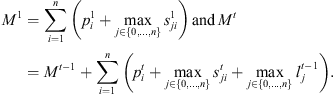 (14)
(14)
Constraint set (6) forces job j at stage t to be completed after its completion at stage t − 1, plus its processing time at stage t, plus the time lag at stage t. The value Mt is set to 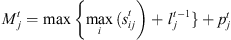 . Constraint sets (5) and (6) together ensure that a job would not begin setup until it is available (done at the previous stage) and the previous job at the current stage is completed. Constraint sets (5) and (6) also serve as sub-tour elimination constraints. Constraint set (7) ensures that jobs that do not visit a stage are not assigned to that stage. Constraint sets (8) and (9) ensure that the completion time of a job at the stage t which is not visited by that job is set to the completion time of the job at the previous stage t − 1. The value Mt is an upper bound on the time stage t which completes processing and has the same usage as defined in constraint set (5). Constraint set (10) links the decision variables
  and z. Constraint sets (11)–(13) provide limits on the decision variables.
3.3. An illustrative numerical example
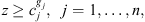
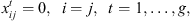
The following examples will help in illustrating this complex HFS problem. We have an instance with four jobs and two stages with one machine in the first stage and two machines in the second stage. Therefore, n = 4, g = 2, m1 = 1, and m2 = 2. The problem data are shown in Tables 1–4.
Processing times  of four jobs at two stages.
Setup times  of four jobs at two stages
Setup times  of four jobs at two stages.
Time lags  of four jobs at two stages.
This example has been solved in four situation and called problem 1, 2, 3, and 4.
Problem 1: setup times are anticipatory and time lags can occur simultaneously.
Problem 2: setup times are non-anticipatory and time lags can occur simultaneously.
Problem 3: setup times are anticipatory and time lags can’t occur simultaneously.
Problem 4: setup times are non-anticipatory and time lags can’t occur simultaneously.
The LINGO 8 software was used to solve these problems and obtain optimal solution. LINGO is a software to make building and solving Linear, Nonlinear, Quadratic, Quadratically Constrained, Second Order Cone, Stochastic and Integer optimization models. It lets you formulate your linear, nonlinear and integer problems quickly in a highly readable form.
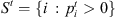
The resulting Gantt charts are shown in Figures 1–4.
 |
Figure 1. Gantt chart for the example problem 1, Cmax = 22. |
 |
Figure 2. Gantt chart for the example problem 2, Cmax = 22. |
 |
Figure 3. Gantt chart for the example problem 3, Cmax = 24. |
 |
Figure 4. Gantt chart for the example problem 4, Cmax = 24. |
Although an optimal solution was obtained for the problem, the computational time was excessive. Attempts to solve larger problems were unsuccessful as they required too much CPU computational time. Hence, a meta-heuristic algorithm is developed to obtain a near-optimal solution for realistic sized problems.
4. Resolution approaches for HFS scheduling problem
4.1. Heuristics
In the HFS scheduling literature, heuristics and exact methods such as branch and bound are the two approaches mostly employed. When we are confronted with the fact that the problem is NP-hard and the optimal solution is unattainable in a reasonable time by exact methods, which are the case of the problem studied in this paper, then it is reasonable to sacrifice optimality and settle for a “good” feasible solution that can be computed efficiently. Of course, we would like to sacrifice as little optimality as possible, while gaining as much as possible in efficiency. Various heuristics have been developed for a scheduling hybrid flow shop without time lags and can be classified in several categories. These include heuristics which rely on specific knowledge of the problem and thus use special properties of the problem: (1) defining priorities among jobs, (2) transforming into simpler problems, such as two-machine problems, (3) using other methods that directly seek a good sequence, such as neighborhood search methods, genetic algorithm and immune algorithm.
In the following subsection, we discuss, develop and compare the performance of heuristic methods based on Johnson (g/2, g/2), SPTCH and Palmer for solving HFS scheduling problem. In all the following heuristics, a modified processing time is used. It is denoted by  for job i in stage t and is defined as
 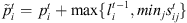 . This time represents the minimum time at stage t that must elapse before job i could be completed.
4.1.1. Johnson’s rule-based heuristic (g/2, g/2)
This heuristic is an extension of Johnson’s rule to take into account the sequence-dependent setup times and time lags. Only the first and last stages are considered to create the order for assignment in stage 1. So,  is the summation of modified processing times for stages 1 to g/2 and
  is the summation of those for stages g/2 + 1 to g. This algorithm includes following steps.
1. Create the modified processing times  , for each stage t = 1, … , g.
2. Calculate processing time summations![Mathematical equation: $$ a.s{\mathop{p}\limits^\tilde}_i^1=\sum_{t=1}^{\left[\frac{g}{2}\right]}{\mathop{p}\limits^\tilde}_i^t $$](/articles/mfreview/full_html/2014/01/mfreview130004/mfreview130004-eq33.gif)
![Mathematical equation: $$ b.s{\mathop{p}\limits^\tilde}_i^2=\sum_{t=\left[\frac{g}{2}\right]+1}^g{\mathop{p}\limits^\tilde}_i^t $$](/articles/mfreview/full_html/2014/01/mfreview130004/mfreview130004-eq34.gif)
3. Let 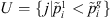 and
and  .
.
4. Arrange jobs in U in non-decreasing order of  and arrange jobs in V in non-increasing order of
  .
.
5. At each stage t = 1, ..., g, assign job 0 to each machine in that stage.
6. For [i] = 1 to n i ∈ S1:
For mc = 1 to m1:
a. Place job [i] in the last position on machine mc
b. Compute completion time of job [i] on machine mc
c. If this placement results in the lowest completion time for job [i], let m = mc
d. Place job [i] in the last position on machine m.
7. For each stage t = 1, …,g:
a. Available time at stage t = completion time at stage t-1
b. Sort jobs in non-decreasing order of available time
c. For [i] = 1 to n, i ∈ St:
I) Place job [i] in the last position on machine mc
II) Compute completion time of job [i] on machine mc
III) If this placement results in the lowest completion time for job [i], let m = mc.
4.1.2. SPT cyclic
This is a naive greedy heuristic that assign jobs to machines with little or no regard for setup times or the interactions between stages. Because of its simplistic nature, it provides a basis of comparison for the other heuristics. In the SPT Cyclic Heuristic (SPTCH), the jobs are ordered at stage 1 in increasing order of the modified processing times  . At subsequent stages, jobs are ordered based on earliest ready time. A job is assigned to a machine in every stage in which the job is allowed to be completed at the earliest time as measured in a greedy fashion as follow.
1. Create the modified processing times  .
.
2. Order the jobs in non-decreasing order (i.e., SPT rule) of  .
.
3. At each stage t = 1; …; g, assign job 0 to each machine in that stage.
4. For stage 1:
a. Let bestmc = 1.
b. For [i] = 1 to n, i ∈ S1:
For mc = 1 to m1:
Place job [i] last on machine mc.
Find the completion time of job [i]. If it is less on mc than on bestmc, let bestmc = mc.
Assign job [i] to the last position on machine bestmc.
5. For each stage t = 2, …, g:
a. Update the ready times in stage t to be the completion times in stage t - 1.
b. Arrange jobs in increasing order of ready times.
c. Let bestmc = 1.
d. For [i] = 1 to n, i ∈ St:
For mc = 1 to mt:
Place job [i] at the last position on machine mc.
Find the completion time of job [i]. If this time is less on mc than on bestmc, let bestmc = mc.
Assign job [i] to the last position on machine bestmc.
4.1.3. Palmer heuristic Algorithm
Palmer heuristic algorithm presented near optimum solution based on slope order of jobs [13]. In this algorithm, jobs which have long processing time on last machines must be located at the beginning of sequence. Slope order index is calculated by equation (15).![Mathematical equation: $$ S{I}_j=-\sum_{i=1}^m\left\{\left[m-\left(2i-1\right)\right]/2\right\}. $$](/articles/mfreview/full_html/2014/01/mfreview130004/mfreview130004-eq42.gif) (15)
(15)
4.2. The proposed Genetic algorithm
Genetic algorithm (GA) is one of the common effective meta-heuristic algorithms, presented by Holland [5], which is started by N feasible initial solution (chromosome) randomly as the population and for each chromosome a fitness function is computed. In each generation, we propose a RKGA. Scheduling data can state in Chromosome shape. Genetic operators are imposed on population with determined probability that can make various shapes on solutions. In our proposed algorithm, each solution is coded as a chromosome and the preferred solution is evaluated based on Cmax.
The genetic operators and related parameters used in this research are based on those in Kurz and Askin [10]. Each generation has a population of 100 chromosomes. The initial population is generated randomly. An elitist strategy is used for reproduction. Each chromosome is decoded and the resulting schedule is evaluated for the makespan. Chromosomes with the lower values of makespan are more desirable, so 20% of the chromosomes with the lowest values of makespan are automatically copied to the next generation. For each chromosome in the next generation, the following is performed. Two chromosomes in the current generation are selected at random. For each job, a random number is generated. If the generated value is less than 0.7 (following Kurz and Askin [10]), the generated value from the “first” chromosome is copied to the new chromosome, otherwise the value from the “second” chromosome is selected. The remaining 1% of the next generation is filled through “immigration”, in which new chromosomes are randomly generated. The above procedures are repeated until we are fairly sure that the population has settled into a good location in the search space. In this research, we continue until 100 generations have been examined without finding an improved schedule. This value was selected empirically.
Deeply view on genetic algorithm is as follow:
1. Initialization:
a. Parameters setting: set the number of initial population (np), number of generation (ng), probability of crossover (pc), probability of mutation (pm).
b. Initial population generation:
b.1. Randomly generate an initial population of (np - 3) antibodies.
b.2. Generate an chromosome with SPTCH.
b.3. Generate an chromosome with palmer.
b.4. Generate an chromosome with g/2, g/2 Johnson’s rule.
2. Evaluate the fitness function for each of the chromosomes.
3. Mating pool generation.
4. Crossover operation: select (np * pc) pairs of parents from mating pool, and perform crossover on the parents at a randomly.
5. Mutation operation: select (np * pm) chromosomes from mating pool, and mutate the individual gens.
6. Fitness evaluation: compute the fitness values for the new population of (np) chromosomes.
7. Termination test: terminate the algorithm if the stopping criterion is met; else return to step 2.
4.2.1. Crossover operator
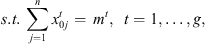
We use the modified OX method. The modified OX method is explained better using two processes, five jobs, two machines in process 1, and three machines in process 2 example. Consider two parents, P1 and P2, with a randomly generated cut point for each process. By exchanging the whole number of the sequences before the cut point, and the integer part of the remained sequences, two clones (or offspring) can be generated as Figure 5, where .xx represents the fractional part that is currently unknown. Starting from the cut point of one parent, the corresponding fractional parts from the other parent are copied one by one.
 |
Figure 5. OX crossover operator example. |
The crossover operator has now generated two clones (or offsprings) from two parents. It can be seen that the clones (or offsprings) share a lot of properties with their parents. Using the modified OX method as the crossover operator, only the job order is allowed to vary. Machine assignment, on the other hand, could not be changed during a crossover operation.
4.2.2. Mutation operator
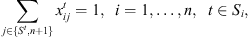
In this research, we propose and use a dual point mutation for each of the processes. A mutation operator is used to exchange the machine assignment and jobs sequencing for two jobs in a particular process. Basically, mutation begins when two random mutation points in the sequences is selected. Then, the real number in mutation points is exchanged (Figure 6).
 |
Figure 6. Dual point mutation operator example. |
This RKGA with proposed crossover and mutation is called RKGAF.
4.2.3. Objective function computation
Typically, an objective function comprises one or more performance indicators that measure the effectiveness of a chromosome or a schedule produced by a GA. The candidate chromosomes are first transformed into valid schedules. On completion, they are evaluated using an objective function to obtain their fitness values. For a maximization problem, a high fitness value is desirable and a GA attempts to maximize it. For a minimization problem, the objective function is formulated in such a way as to transform it into a maximization problem. In our case, the makespan is to be minimized; a candidate solution with a high makespan is assigned a low fitness value [4]. Here, for chromosome i, it is calculated as follows:
where f(i) is the fitness value for chromosome i, Cmax(i) is the makespan for chromosome i, and N is the population size.
5. Computational evaluation
This section describes the computational tests which are used to evaluate the performance of the presented algorithms. For this reason, various testing problems of hybrid flow shop scheduling are generated randomly. The testing problems are divided to two categories: small-sized hybrid flow shop scheduling problems (SHFS1:10) and medium and large-sized hybrid flow shop scheduling problems. Each problem has integer processing times selected from a uniform distribution between 50 and 70 and integer setup times and time lags selected from a uniform distribution between 12 and 24 [14].
The mathematical model, the MILP model presented in Section 4, is coded by LINGO 8 software which solves the model by the branch and bound method. The branch and bound method is a traditional optimization technique which obtains the optimum solution. These test problems are also solved by the proposed algorithms to evaluate their effectiveness and efficiency. For this purpose, we coded the proposed algorithms by MATLAB 7.5. This program and the LINGO software were run on a PC that has a Pentium IV with 2 GHz processor, and 1024 Mb RAM. All of the test problems are solved by the proposed algorithms and the branch and bound method. Their results are shown in Table 5, which shows the test problems specification, the results of the branch and bound method and the results of the proposed algorithm. Following Fattahi et al. [2], to evaluate solutions, a factor is used, namely,  which determines the mean deviation of the best solution. This factor is described below, in which f* denotes the best solution in 14 runs and n is the number of runs. A summary of results in Table 5 shows that the proposed algorithm is capable of attaining a solution near the optimal solution.
Aggregated results for the heuristic and IP model in small size.
To verify the heuristics and meta-heuristic algorithm in medium and large-size hybrid flow shop scheduling problems, some data are generated. The testing problems are determined by size of the problem (n.g) in which index n denotes the number of jobs and g denotes the number of stages. Processing time and setup time for each job are distributed as a U [20, 100] and 20–40% of the average of processing time, respectively. Also, time lag is distributed as a U [12, 24]. Based on flexible job shop conditions, some jobs can jump to some stages with the probability of 0.1. Problems data are divided into seven categories which are shown in Table 6.
Factor levels.
For each factor, 27 scenarios are introduced and for each scenario 10 sample problem are generated, so, totally, 270 sample problems are generated. For GA, 10 problems for each n (30 sample problems) are generated. In addition to population size, experimental design for three genetic operators is also done. These values for copy, mutation and crossover rate are mentioned as 15%, 5% and 80%, respectively. The extended heuristics and meta-heuristic algorithm are implemented in MATLAB 7.5 and run on a PC with a Pentium IV 2000 MHz processor with 1024 MB of RAM. To evaluate the performance of heuristics and compare them, stop criterion is equal to 500. While 270 sample problems are solved, the best solution obtained by heuristic algorithms are mentioned as Minsol and the best solution obtained by meta-heuristic algorithms are mentioned as Algsol. Furthermore, Relative Percentage Deviation (RPD) is calculated by equation (17). (17)
(17)
To evaluate described algorithms in different sizes, average of relative deviation of 160 sample problems is shown in Table 7.
RPD for Algorithms in different sizes.
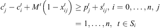
As results demonstrate, Johnson with 12.06% RPD has the best performance among the heuristics. In contrary, RKGAF with the performance rating of 0.07% RPD has the best results among all the proposed algorithms. Furthermore, analysis of variance (ANOVA) test for better analysis is done by SPSS14 software. It is concluded that Johnson is better than the other extended heuristics and RKGAF is the best among all the proposed algorithms (less relative percentage deviation). It is shown graphically in Figure 7.
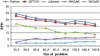 |
Figure 7. Graphically presentation of performance evaluation of algorithms |
6. Conclusions and future work
In this paper, the hybrid flow shop scheduling which considers some real constraints in real world and a formulation as well as an integer linear programming mathematical model is presented. In this problem, three realistic characteristics are jointly considered. These include time lags between jobs, sequence-dependent setup times and possibility for jobs to skip stages. To the best of our knowledge, such a complex problem has not been considered so far. This modeling allows for the consideration of complex scheduling environments like those arising in the production of prepared food, ceramic tiles, wood processing, and in the manufacture of furniture, as well as many others.
Whereas, solving such problems in large size is time-consuming and costly, we proposed meta-heuristic genetic algorithm in addition to three heuristics. Evaluation, discussion and comparison are also done and it is concluded that Johnson is a preferred algorithm among other heuristics and GA has the best performance among all other heuristics (with the less RPD).
The experiment results show the effectiveness of the proposed algorithm. The proposed algorithm can reach better results compared with the algorithm presented by Kurz and Askin [10] (RKGA). In this paper, an immune algorithm is used to solve the considered problem. Solving this problem using other metaheuristic algorithms can be suggested for further research. Also, developing a multi-objective approach to present the Pareto optimal solutions can be suggested for further research.
There are potentially unlimited opportunities for research in scheduling to minimize makespan in hybrid flow shops with time lags and sequence-dependent setup times. In this paper, we have addressed only a few areas. By creating a general permutation schedule definition, we may be able to find a class of schedules that contains the optimal makespan schedule for some special cases, such as two stages with one machine at the first stage and two machines at the second, with sequence-dependent setup times at both.
References
- V. Botta-Genoulaz, Hybrid flow shop scheduling with precedence constraints and time lags to minimize maximum lateness, International Journal of Production Economics 64 (2000) 101–111. [CrossRef] [Google Scholar]
- P. Caricato, A. Grieco, D. Serino, Tsp-based scheduling in a batch-wise hybrid flow-shop, Robotics and Computer-Integrated Manufacturing 23 (2007) 234–241. [CrossRef] [Google Scholar]
- P. Fattahi, M. Saidi, F. Jolai, Mathematical modeling and heuristic approaches to flexible job shop scheduling problems, Journal of Intelligent Manufacturing 18 (2007) 331–342. [CrossRef] [Google Scholar]
- J. Fondrevelle, A. Oulamara, M.-C. Portmann, Permutation flow shop scheduling problems with maximal and minimal time lags, Computers & Operations Research 33 (2006) 1540–1556. [CrossRef] [MathSciNet] [Google Scholar]
- D.E. Goldberg, Genetic algorithms in search optimization and machine learning, Addison-Wesley, Reading, MA, 1989. [Google Scholar]
- J.H. Holland, Adaptation in Natural and Artificial Systems, The University of Michigan Press, Ann Arbor, 1975. [Google Scholar]
- T.S.L. Hung, J.L. Ching, A case study in a two-stage hybrid flow shop with setup time and dedicated machines, International Journal of Production Economics 86 (2003) 133–143. [CrossRef] [Google Scholar]
- N. Javadian, P. Fattahi, M. Farahmand-Mehr, M. Amiri-Aref, M. Kazemi, An immune algorithm for hybrid flow shop scheduling problem with time lags and sequence dependent setup times, International Journal of Advanced Manufacturing Technology 63 (2012) 337–348. [CrossRef] [Google Scholar]
- M.E. Kurz, R.G. Askin, Comparing scheduling rules for flexible flow lines, International Journal of Production Economics 85 (2003) 371–388. [CrossRef] [Google Scholar]
- M.E. Kurz, R.G. Askin, Scheduling flexible flow lines with sequence-dependent setup times, European Journal of Operational Research 159 (2004) 66–82. [CrossRef] [MathSciNet] [Google Scholar]
- R. Logendran, P. de Szoeke, F. Barnard, Sequence dependent group scheduling problems in flexible flow shops, International Journal of Production Economics 102 (2006) 66–86. [CrossRef] [Google Scholar]
- B.A. Norman, J.C. Bean, A genetic algorithm methodology for complex scheduling problems, Naval Research Logistics 46 (1999) 199–211. [CrossRef] [MathSciNet] [Google Scholar]
- D. Palmer, Sequencing jobs through a multi-stage process in the minimum total time a quick method of obtaining a near optimum, Operational Research Quarterly 16 (1965) 101–107. [CrossRef] [Google Scholar]
- R.Z. Rios-Mercado, J.F. Bard, Computational experience with a branch-and-cut algorithm for flow shop scheduling with setups, Computers and Operations Research 25 (1998) 351–366. [CrossRef] [Google Scholar]
- R. Ruiz, C. Maroto, A genetic algorithm for hybrid flow shops with sequence dependent setup times and machine eligibility, European Journal of Operational Research 169 (2006) 781–800. [CrossRef] [MathSciNet] [Google Scholar]
- R. Ruiz, C. Maroto, J. Alcaraz, Solving the flow shop scheduling problem with sequence dependent setup times using advanced metaheuristics, European Journal of Operational Research 165 (2005) 34–54. [CrossRef] [MathSciNet] [Google Scholar]
- M. Zandieh, S.M.T. FatemiGhomi, S.M. MoattarHusseini, An immune algorithm approach to hybrid flow shops scheduling with sequence-dependent setup times, Applied Mathematics and Computation 180 (2006) 111–127. [CrossRef] [MathSciNet] [Google Scholar]
Cite this article as: Farahmand-Mehr M, Fattahi P, Kazemi M, Zarei H & Piri A: An efficient genetic algorithm for a hybrid flow shop scheduling problem with time lags and sequence-dependent setup time. Manufacturing Rev. 2014, 1, 21.
All Tables
All Figures
|
Figure 1. Gantt chart for the example problem 1, Cmax = 22. |
| In the text | |
|
Figure 2. Gantt chart for the example problem 2, Cmax = 22. |
| In the text | |
|
Figure 3. Gantt chart for the example problem 3, Cmax = 24. |
| In the text | |
|
Figure 4. Gantt chart for the example problem 4, Cmax = 24. |
| In the text | |
|
Figure 5. OX crossover operator example. |
| In the text | |
|
Figure 6. Dual point mutation operator example. |
| In the text | |
|
Figure 7. Graphically presentation of performance evaluation of algorithms |
| In the text | |
Current usage metrics show cumulative count of Article Views (full-text article views including HTML views, PDF and ePub downloads, according to the available data) and Abstracts Views on Vision4Press platform.
Data correspond to usage on the plateform after 2015. The current usage metrics is available 48-96 hours after online publication and is updated daily on week days.
Initial download of the metrics may take a while.