| Issue |
Manufacturing Rev.
Volume 13, 2026
|
|
|---|---|---|
| Article Number | 9 | |
| Number of page(s) | 21 | |
| DOI | https://doi.org/10.1051/mfreview/2025029 | |
| Published online | 27 February 2026 | |
Review
Pre-formed metal membranes for diaphragm compressors: a combined numerical and experimental investigation of forming process and fatigue life
1
Professorship Forming Technology, Institute for Machine Tools and Production Processes, Chemnitz University of Technology, 09126 Chemnitz, Germany
2
Fraunhofer Institute for Machine Tools and Forming Technology IWU, Chemnitz, Germany
* e-mail: This email address is being protected from spambots. You need JavaScript enabled to view it.
Received:
15
August
2025
Accepted:
15
November
2025
Abstract
Conventional diaphragm compressors are fundamentally limited by the low displaced volume and poor fatigue life of their flat metal diaphragms. This study presents a comprehensive, numerical and experimental investigation of the design, manufacturing, and performance of pre-formed, bistable dome-shaped membranes to overcome these limitations. A complete process chain was modeled using the finite element method (FE), simulating the hydroforming process, subsequent elastic springback, and the operational folding cycle. The model was based on the characterization of the anisotropic material properties of high-strength stainless steel foil made of 1.4310 in a spring-hard condition. To validate the simulation, prototypes were manufactured via hydroforming and their final geometries were analyzed using an optical 3D scanning system, showing improved results using the anisotropic material model compared the isotropic. X-ray diffraction (XRD) analysis was applied to quantify induced martensite transformation as part of the material hardening behavior. Subsequent, fatigue life testing was performed on the manufactured membranes to assess their durability under cyclic loading. The results demonstrate that the hydroforming process yields a robust component with superior performance. The optimized hydroformed diaphragm successfully endured over 5 million cycles without failure and enabled an increase of 60% in displaced volume compared to a conventional flat membrane. This integrated design and validation methodology provides a clear pathway for developing next-generation, high-performance diaphragm compressors.
Key words: Diaphragm compressor / metal membrane / metal forming / finite element simulation / fatigue life
© M. Solovev et al., Published by EDP Sciences, 2026
 This is an Open Access article distributed under the terms of the Creative Commons Attribution License (https://creativecommons.org/licenses/by/4.0), which permits unrestricted use, distribution, and reproduction in any medium, provided the original work is properly cited.
1 Introduction
The global transition towards sustainable energy systems has positioned hydrogen as a cornerstone for decarbonizing various sectors, including transportation, industry, and energy storage [1,2]. A critical enabling technology for the hydrogen economy is the efficient and safe compression of hydrogen gas, which is essential for its storage in high-pressure vessels (e.g., 350 to 700 bar) and its distribution, particularly for hydrogen refueling stations (HRS) [3,4].
The selection of an appropriate compressor technology is paramount and depends heavily on the application-specific requirements for gas purity, pressure levels, and leakage integrity. Generally, compressors can be categorized into dynamic and positive displacement types. While dynamic compressors, such as turbo compressors, are suitable for high flow rates at lower pressure ratios, positive displacement compressors, like piston, screw, and diaphragm compressors, are preferred for high-pressure applications [5]. Piston and screw compressors are widely used but often rely on oil for lubrication and sealing, which introduces the risk of contaminating the process gas being a critical issue for high-purity applications like fuel cells. While non-lubricated variants exist, they may still face challenges regarding wear and internal leakage, affecting efficiency and maintenance requirements [6].
In this context, diaphragm compressors have carved out a crucial niche. Their unique design, which uses a metallic or elastomeric diaphragm to separate the process gas from the hydraulic drive mechanism, ensures hermetic sealing and completely oil-free, contamination-free compression [7]. These characteristics are the reasons why diaphragm compressors are the technology of choice for compressing high-purity, toxic, reactive, or explosive gases, with hydrogen being a primary example [8,9]. However, despite their advantages, conventional diaphragm compressors, which utilize flat metal diaphragms, are constrained by two major limitations: a relatively low flow rate and, most critically, a limited fatigue life of the diaphragm itself. A schematic of a conventional diaphragm compressor is shown in Figure 1. Previous research has extensively investigated the failure mechanisms of flat diaphragms, identifying stress concentrations at the cavity center and the clamping edge, as well as the overall cavity profile, as the main drivers for premature fatigue failure and fracture [11, 12]. Studies have focused on optimizing the cavity profile to achieve a more uniform stress distribution and on material selection to enhance durability, but the inherent trade-off between diaphragm displacement (flow rate) and mechanical stress remains a fundamental challenge [13, 14].
To overcome these limitations, recent research has shifted focus from optimizing the operation of flat diaphragms to redesigning the diaphragm itself. Previous work initiated the concept of using pre-formed, bistable, elastically deformable metal membranes to increase the displaced volume per stroke. Bistable structures are a class of deployable systems characterized by the ability to maintain two distinct, stable geometric states without the need for external constraints. These states typically consist of a compact, coiled configuration for efficient transport and storage, and a deployed, functional geometry, such as a long supporting shell. This bistability in thin, high-strength metallic shells is achieved by strategically inducing a specific residual stress distribution through the material's thickness. Bistability was investigated in [15] in order to produce tubes using a sequence of two plastic bending steps (incremental die bending), which were applied in opposite directions along two perpendicular axes. This process creates a tailored internal stress state that determines the two stable equilibrium shapes of the final component. In [16], various bistable membrane geometries (e.g., cone, dome) for diaphragm compressors were introduced and numerically investigated, which were then manufactured using Single Point Incremental Forming (SPIF). This initial study demonstrated the potential of pre-formed diaphragm to significantly increase the displaced volume but also highlighted the impact of the forming process on the fatigue life due to induced surface topology and residual stresses. Subsequently, alternative forming technologies, hydroforming and stretch forming, were applied to manufacture pre-formed membrane from the high-strength stainless steel 1.4310. A dome-shaped membrane was produced by hydroforming with twice the volume of a flat diaphragm. This membrane exhibited a vastly superior fatigue life of over 5 million cycles, demonstrating the critical link between the forming process and the final performance of the component [17]. Central to these material properties is the significant hardening that occurs during forming. The strain-induced transformation from austenite to martensite is a well-documented phenomenon in metastable stainless steels like 1.4310 and 1.4404 during cold forming. This transformation significantly alters the local mechanical and electrochemical properties, which is why its quantification is critical for understanding the final performance of the formed component. [18]
The present study aims to provide a comprehensive and systematic investigation of the relationship between the manufacturing process, the resulting material properties, and the operational fatigue life of pre-formed metal membranes. A combined numerical and experimental approach was applied to: (1) develop a validated, coupled finite element (FE) model that simulates both the forming process (hydroforming) and the subsequent cyclic elastic deflection (springback), (2) experimentally manufacture membranes and characterize their geometry and microstructure properties, and (3) conduct extensive fatigue life testing to quantify the performance. By establishing a clear process-structure-property relationship, this work seeks to provide a robust methodology for the design and manufacturing of high-performance, long-life membranes, thereby addressing a key bottleneck in advancing diaphragm compressor technology for the hydrogen economy and other demanding applications.
2 Approach: Pre-formed membranes for diaphragm compressors
The fundamental limitation of conventional diaphragm compressors is caused by the performance of the flat diaphragm. A conventional flat membrane deflects elastically in both directions from a neutral center plane, as shown in Figure 1. As illustrated in Figure 2a, a flat metal membrane has a stroke volume (Vflat) that is solely determined by its elastic deflection (2·Velast1) when subjected to the operating pressure differential. To maximize this displaced volume, the pressure has to be increased, which inevitably leads to higher mechanical stresses and a reduced fatigue life, creating a restrictive trade-off between performance and durability.
To overcome these limitations, a new approach in designing the metal membrane is proposed: pre-formed, bistable metal membranes instead of flat sheets. The pre-formed membrane is bistable and deflects between a pre-formed state on the one side (in forming direction) and a resulting state on the other side (opposite to forming direction). The basic principle is to introduce a defined plastic deformation during a manufacturing step to create a non-flat, three-dimensional geometry (e.g., a dome or cone). This concept is schematically depicted in Figure 2b.
The total stroke volume of a pre-formed membrane (Vpre-formed) in one direction contains two sub-volumes:
The volume Vplast due to the plastically pre-formed geometry of the membrane.
The volume Velast2 which is generated by the elastic deflection of the pre-formed geometry during the compression cycle.
The resulting stroke volume Vpre-formed can be expressed as:
 (1)
(1)
assuming that both directions show identical deflection behavior. This is a simplification, as only one direction is actually preformed.
This approach offers an increase of the displaced volume per stroke which is larger than the purely elastic deflection of a flat membrane: Vpre-formed > Vflat. The key factor that enables and limits the displaced volume of the pre-formed membrane is the elastic deformation characteristic of the material. Due to the forming process (plastic deformation), material hardening can be observed in the stress-strain curve in Figure 2c which is initiated by strain hardening and martensite formation in case of the used austenitic stainless steel 1.4310. The material hardening causes:
An increase in the flow stress kf to initiate plastic deformation of the material kf_pre-formed compared to the flow stress of the flat membrane kf_flat.
An increase in the elastic deformation potential εelast2 compared to εelast1 of the flat membrane.
The hardened material (1) allows higher stress states without plastic deformation during deflection of the pre-formed membrane which only has to be performed in the elastic range to not affect the fatigue life. This directly affects Vplast which should be maximized within the limitation of an elastic deflection. The higher elastic range due to the hardening also influences Velast2 which additionally depends on the external pressure load. The operational cycle of the pre-formed membrane has to be designed to occur entirely within this extended elastic region, ensuring purely elastic deflection during operation and thus a long fatigue life.
This leads to the central research question guiding this study: How can the geometry and the manufacturing process of the membrane be optimally designed to maximize the displaced volume (Vpre-formed) while ensuring the operational deflection remains purely elastic to guarantee a sufficient service life? To address this question, this study combines numerical simulation of the forming and deflection processes with experimental validation through prototype manufacturing and fatigue life testing.
 |
Fig. 2 Solution approach: Increase in stroke volume due to plastic deformation and hardening of the membrane: a) conventional, flat membrane (max. deflection under 0.1 bar –3.2 mm), b) pre-formed membrane (max. deflection under 0.1 bar –6.76 mm) and c) utilization of the hardening by forming. |
3 Material characterization for pre-formed membranes
3.1 Material selection for pre-formed membranes
The selection of a suitable material is critical for the successful implementation of pre-formed diaphragms, as it must balance the requirements of manufacturability (sufficient ductility for plastic forming) with operational performance (high yield strength and fatigue resistance). A review of established materials for diaphragm compressors reveals a strong preference for metallic membranes, especially for high-purity and high-pressure applications such as hydrogen compression, where hermetic sealing and non-contamination are paramount [7, 8].
Conventional diaphragm compressors commonly utilize high-strength spring materials in hardened condition (spring-hard condition). A widely adopted standard is the austenitic stainless steel 1.4310 (X10CrNi18-8; AISI 301), which provides a favorable combination of mechanical properties, corrosion resistance against a wide range of media, and formability [6,19]. For more demanding applications involving highly corrosive gases or extreme temperatures, specialized alloys such as Hastelloy, Inconel, or duplex steels are employed [5,6]. Some designs also utilize copper-beryllium alloys for their superior mechanical characteristics [6]. The diaphragms are often constructed as a three-layer “sandwich” assembly, where a slotted middle layer acts as a signal membrane for rupture detection, enhancing operational safety [6,20].
For this study, austenitic stainless spring steel 1.4310 was selected as the diaphragm material. The choice was driven by several key factors:
Hardening potential by forming: As a metastable austenitic steel, the hardening behavior of 1.4310 is defined by work-hardening and induced martensite formation. Therefore, this stainless steel exhibits significant hardening upon plastic deformation, like cold rolling [18] and hydroforming. This property is central to the solution approach, as the pre-forming process can be used to substantially increase the flow stress, thereby creating a larger elastic operating range for the finished membrane (as illustrated in Fig. 2).
Proven performance: This material is well-established and has a proven track record in conventional diaphragm compressors, providing a solid baseline for comparison and demonstrating its fundamental suitability for the demanding cyclic loading conditions.
Hydrogen compatibility: While hydrogen embrittlement is a concern for many high-strength steels, austenitic stainless steels like 1.4310 are generally considered to have sufficient resistance, especially in the temperature ranges typical for diaphragm compressor operation. Some literature also cites the use of similar grades like 316L for hydrogen-wetted components, reinforcing this choice [6]. However, the formation of martensite has to be taken into account for the application in hydrogen environment.
Therefore, a cold-rolled 1.4310 foil with a thickness of 0.1 mm and a yield strength in the range of 1500–1700 MPa was used within this work.
3.2 Characterization of mechanical properties
The mechanical properties (e.g. flow curve, anisotropy) of the as-received 1.4310 stainless steel foil (thickness 0.1 mm, strength grade 1500–1700 MPa) were comprehensively characterized through uniaxial tensile tests as input for the FE simulations.
Tensile specimens according to DIN EN ISO 6892-1 were prepared in three different orientations relative to the rolling direction (RD): 0° (longitudinal), 45° (diagonal), and 90° (transverse) to determine the anisotropy resulting from the cold-rolling process. The initial specimen blanks were cut from the foil using an abrasive waterjet cutting process to minimize thermal effects. Subsequently, the samples were stacked and the edges of the specimens were milled to achieve a high-quality surface finish and remove any potential micro-cracks or hardened zones from the initial cutting step, ensuring that failure initiation would occur within the gauge length.
Uniaxial tensile tests were performed according to DIN EN ISO 6892-1. For each of the three orientations (0°, 45°, 90°), five tensile tests were conducted. The deformation was monitored using a non-contact, optical 3D deformation analysis system (ZEISS GOM Aramis) during testing. This full-field measurement technique allowed for the precise determination of true stress-true strain curves by accurately capturing the local strain distribution and the onset of necking. Besides the flow curve, the Young's modulus, the Poisson's ratio and the r-values have been determined from the tensile tests.
3.3 Flow curve fitting and extrapolation
The experimentally obtained true stress-true strain data from the tensile tests in Figure 3a served as the basis for the constitutive material model used in the FE simulation. Since the plastic strains occurring during the forming process can exceed those reliably measured in a tensile test, the experimental flow curves required extrapolation. In case of the used stainless steel foil, true strains below 0.1 have been achieved within the tensile tests in the three different directions. The flow curves presented in Figure 3a represent the average curves of the five tensile tests in each direction. The true strain value did not reach 0.01 in case of the tensile samples in 0° to RD, although the sample preparation has been optimized by milling the edges and different batches have been analyzed. Therefore, the flow curves in 45° and 90° to RD have been used to identify a suitable extrapolation approach. These flow curves show a characteristic progress which has a high slope at the beginning and a reduced slope after a specific strain value. A combined Swift-Voce modeling approach was chosen to accurately describe and extrapolate the hardening behavior of the stainless steel foil also for larger true strain values [20]. This was achieved by fitting established hardening models to the experimental data using the software OriginPro. For the initial region of plastic deformation, characterized by a high hardening, the Swift hardening law was applied [21]:
 (2)
(2)
where σswift is the true stress, ε is the true plastic strain, K is the strength coefficient, n is the strain hardening exponent, and ε0 is a true plastic pre-strain offset.
To describe the material behavior at higher strains, where the hardening decreases and approaches saturation, the Voce hardening law was used for εt > 0.0077 (0° and 90°) and εt > 0.00595 (45°) [22]:
 (3)
(3)
where σsat is the saturation stress, and A and C are material parameters that define the shape of the saturation curve.
The parameters for both the Swift and Voce models were determined for each material orientation (0°, 45°, and 90°) using the non-linear curve fitting capabilities of OriginPro. A hybrid hardening law was employed to describe the plastic flow behavior. The initial stage of hardening was described by the Swift equation up to a transition strain εt. Beyond this point, the Voce equation was used to model the subsequent saturation behavior. While the Swift parameters were determined independently for each orientation, a convergent fit for the Voce constants (σsat, A, C) could not be achieved in the 0° direction because of the small strain at fracture. As an assumption, the Voce parameters derived from the 90° orientation were also applied for 0°. The calculated fitting parameters are summarized in Table 1.
Based on these fitted parameters, the flow curves were extrapolated to the higher strain levels expected during the forming simulation. The resulting flow curves, shown in Figure 3b, clearly indicate the anisotropic behavior of the used material, with the highest flow stress observed in the 0° direction.
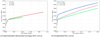 |
Fig. 3 Experimentally determined (average) (a) and extrapolated (b) flow curves of the 1.4310 stainless steel foil. |
Fitting parameters for the hybrid flow curve description.
3.4 Anisotropic material properties
Anisotropic material behavior for the 1.4310 foil was observed in both the elastic and plastic properties determined from the tensile tests. The elastic properties showed a clear directional dependency. The Young's modulus was determined to be E0 = 177.9 GPa in the rolling direction and E90 = 196.2 GPa in the transverse direction. Similarly, the Poisson's ratio was measured as v0 = 0.264 and v90 = 0.385, respectively.
Based on these experimental in-plane data, a full orthotropic elastic model was defined for the FE simulation. The engineering constants for the principal directions were set as follows:
Young's moduli:
 ,
,  .
.Poisson's ratios: v12 = 0.264, v23 = 0.385.
Since the material properties in the through-thickness direction cannot be directly determined from uniaxial tensile tests on thin foils, standard assumptions were made to complete the material card. The through-thickness Young's modulus was assumed to be equal to that of the rolling direction (E3 = E1), and the corresponding Poisson's ratio was assumed to be v13 = v12. The shear moduli G12, G13, and G23 were subsequently calculated using the full set of elastic constants based on the theoretical relationships for orthotropic materials, as shown in the following equations:
 (4)
(4)
 (5)
(5)
 (6)
(6)
To incorporate the observed plastic anisotropy into the FE simulation, the Hill48 anisotropic yield criterion was employed. Under plane stress conditions, the Hill48 yield function f is defined as [23]
 (7)
(7)
where σ¯ is the equivalent stress, and F, G, H, and N are material parameters that describe the anisotropy. These parameters can be determined from experimental data using different methods.
There are two primary approaches for parametrization of the Hill48 anisotropic yield criterion [23]: the stress method, which relies on the initial yield stresses (σ) measured in different directions, and the r-value method, which is based on the Lankford coefficients. Due to the premature failure of the 0° tensile specimens, which led to a high uncertainty in the r0-value and the flow curve at larger strains, both methods were initially considered:
– The parameters of Hill48 yield function based on stress method (Hill48-stress) are as follows:
 (8)
(8)
 (9)
(9)
 (10)
(10)
 (11)
(11)
where σ0, σ90, σ45 and σb are the initial yield stresses in rolling direction, transverse direction, 45° to the rolling direction and the biaxial tension, respectively.
The experimentally determined values were σ0 = 1574 MPa, σ45 = 1445 MPa, and σ90 = 1438 MPa. The biaxial yield stress σb was not measured and was assumed to be equal to the reference yield stress for the calculation.
– The parameters of Hill48 yield function based on the r-values (Hill48-r) are as follows:
 (12)
(12)
 (13)
(13)
 (14)
(14)
 (15)
(15)
where r0, r45 and r90 are the r-values (strain ratios) under uniaxial tensile test in 0°, 45° and 90° to the rolling direction, respectively.
The r-value was measured for all three specimen orientations (0°, 45°, and 90°). The average r-values determined were: r0 = 0.554, r45 = 0.862, r90 = 1.077. It should be noted that the r-value in 0° to the rolling direction was not determined in accordance with the standard. According to standard, the r-values are determined in the range of 2 to 6% elongation. For the 0° orientation, only 1.3% elongation was achieved.
In the FEM software Abaqus, anisotropic yield behavior is modeled based on Hill48 yield function. Anisotropic plasticity potential of Hill48 yield function is defined in Abaqus by the ratios of the anisotropic yield stresses (Rij). These Rij values can be calculated from either the r-values or the initial yield stresses using following equations:
 (16)
(16)
 (17)
(17)
 (18)
(18)
 (19)
(19)
where R11, R22, R33 and R12 are specified material parameters for using Hill48 yield function in Abaqus FEM software.
To investigate the sensitivity of the model to the input data, a single-element FE simulation under uniaxial tension was performed using both parametrization approaches. The input date are summarized in Table 2.
These parameters, along with the directionally dependent Young's modulus, Poisson's ratios and flow curve for 0° or 90° orientation, provide a complete data set for an anisotropic material model.
For the purpose of comparison and to highlight the importance of considering anisotropy, a simplified isotropic material model was also defined. For this model, all elastic and plastic properties were based exclusively on the experimental data from the 90° (transverse) direction. Specifically, the isotropic model was defined with a Young's modulus of E = 196.2 GPa, a Poisson's ratio of v = 0.385, and the plastic hardening behavior described by the 90° flow curve. This allows for a direct, quantitative comparison of the predictive accuracy and demonstrates the effect of anisotropy on the forming and springback behavior.
Material parameter sets used in the single-element analysis.
3.5 Characterization of phase fractions by XRD
The steel 1.4310 used in this study is a metastable austenitic stainless steel, which is known to undergo a strain-induced phase transformation from austenite (fcc) to α′-martensite (bcc/bct) during cold forming [24]. This transformation significantly influences the mechanical properties, particularly its hardening behavior, and, therefore, also the deflection properties of the final membrane. To quantify the extent of this transformation and its distribution across the formed component, a phase analysis was conducted for the initial material as well as for various areas of the formed membranes (see 5.6). Samples were prepared from the flange and the wall area of the dome as well as from the dome pole to investigate the influence of strain on transformation of martensite (Fig. 4a). The samples had a size of approximately 30 mm x 40 mm.
The volume fractions of retained austenite and strain-induced α′-martensite in each specimen were determined using X-ray diffraction (XRD). The measurements were performed using a Bruker Discover D8 diffractometer with Cu-Kα radiation (λ = 0.154 nm) from the top side of the sheet samples, as shown in Figure 4b. The volume fractions of retained austenite and strain-induced α′-martensite were quantified using the Rietveld refinement method applied to the measured X-ray diffraction data. The results of this analysis provide critical insight into the local material state after forming, which is essential for understanding the subsequent performance during cyclic loading.
 |
Fig. 4 Position of samples taken from a hydroformed membrane (a) and the Bruker Discover D8 diffractometer used for quantifying phase fractions (b). |
4 Methods
4.1 Single-element FE simulation
As discussed in Section 3.4, the parametrization of the Hill48 yield criterion can be based on either the Lankford coefficients (r-values) or the initial yield stresses. Due to the uncertainty associated with the experimentally determined r0-value, an analysis was conducted to evaluate the influence of the parametrization method on the predicted material behavior under a uniaxial load case.
For this purpose, a single-element FE model was created in Abaqus, as shown in Figure 5. The model consists of a single C3D8R solid element (a cube with 1 mm side length). To simulate a uniaxial tension state, displacement boundary conditions were applied. The element was stretched in one principal direction (x-direction in Fig. 5), while symmetry boundary conditions were applied to the opposing face (Y-Z-plane) and two corresponding faces (X-Y- and X-Z-plane).
Four distinct anisotropic material definitions were implemented and compared in this model, as summarized in Table 2. These cases explore the two primary parametrization methods (based on r-values vs. based on initial yield stresses) and two different choices of the reference flow curve: flow curve in rolling direction (0° flow curve) and flow curve transverse to rolling direction (90° flow curve). Both were extrapolated according to Section 3.3.
 |
Fig. 5 Single-element model in Abaqus. |
4.2 Numerical simulation of membrane hydroforming and deflection using an anisotropic material model
A three-dimensional (3D) finite element model was set up and solved using the commercial software Abaqus/Standard with an implicit solver to investigate the forming process and predict the operational performance of the membranes. The simulation was designed as a multi-step analysis to capture the plastic deformation during forming, the subsequent elastic springback, and the final (elastic) deflection under operational pressure. The material behavior of the 1.4310 steel foil was described using an anisotropic elastic-plastic model to accurately account for the directionally dependent properties observed in the tensile tests. The material parameters used are described in 3.4.
As depicted in Figure 6, a 3D quarter model of the circular blank and the forming tools (die, blank holder) was created to leverage the geometric symmetry and reduce computational cost. Symmetry boundary conditions were applied accordingly. The model represents a membrane with an active radius of R = 70 mm. The deformable membrane (blank) was meshed with four-node shell elements (S4R) with an average element size of 1 mm, which was found to provide an appropriate compromise between accuracy and computation time in a prior mesh convergence study. Five integration points were set over the thickness of the workpiece. The forming tools were modeled as analytical rigid surfaces. Contact between the membrane and the rigid tools was defined using a standard surface-to-surface formulation with a penalty-based algorithm. A constant friction coefficient of μ = 0.2 was assumed.
The plastic behavior was modeled using the Hill'48 anisotropic yield criterion combined with isotropic hardening. The yield potential was defined using the calculated yield stress ratios (Rij) derived from the experimental Lankford coefficients (r-values) as described in Section 3.4. The isotropic hardening behavior was described by providing the tabulated true stress vs. true plastic strain data from the 0° tensile test as input.
The simulation was performed in a sequence of three distinct steps:
Forming: In this step, the sheet hydroforming was simulated. A uniformly distributed pressure load was applied to one side of the membrane blank (Top plane), gradually increasing from zero to a final forming pressure in the range of 10 to 21 bar. This step was used to investigate the influence of the hydroforming pressure on the plastic deformation of the foil material.
-
Springback: The forming loads were removed, and the model was allowed to reach a new equilibrium. This step was crucial for predicting the final, sprung-back geometry of the membrane, which can deviate significantly from the tool geometry. Furthermore, the true strain and true stress state was evaluated after springback. Therefore, the equivalent plastic strain (PEEQ in Abaqus), the plastic strain (PE in Abaqus) and the elastic strain (EE in Abaqus) as well as the equivalent von Mises stress were analyzed. The equivalent plastic strain
 is defined as:
 (20)
(20)where t is the time and
 is the plastic strain rate tensor.
 Operational deflection: The deflection of the membrane for a two-stroke cycle was simulated in the final step. As a low-pressure actuation of the membrane was intended, a pressure of 0.1 bar was applied. The deflection simulation was performed in the forming tool set-up, i.e. that no cavities restricted the folding of the membranes in both directions in the simulation. A uniform pressure difference of 0.1 bar was applied to the sprung-back geometry from the Base plane to simulate the first deflection in the opposite direction with regard to the forming process. Subsequently, this load was transferred to the opposite Top plane of the membrane to induce the reverse deflection which corresponds to the forming direction. For both strokes, the equivalent plastic strain (PEEQ in Abaqus) was monitored by using the output parameter AC YIELD to verify if the deflection is purely elastic. The AC YIELD parameter is zero for a PEEQ value of zero. If the PEEQ is larger than zero, AC YIELD will show a value of one. Furthermore, equivalent von Mises stress was evaluated during deflection.
This simulation approach provides a holistic view on the process chain, enabling a direct correlation between manufacturing parameters, the resulting part properties, and the final operational performance of the diaphragm. For a quantitative analysis of the anisotropic behavior, the simulation results were post-processed by extracting field output variables (stress and strain) along two orthogonal paths, as shown in Figure 6. Path A was defined from the center to the edge along the rolling direction (0°, corresponding to the Z-axis of the coordinate system and to the 11-direction of the material model), while Path B was defined along the transverse direction (90°, corresponding to the X-axis of the coordinate system and the 22-direction of the material model). The results were evaluated for the Base plane as standard and compared to the values of the Top plane for specific instances.
 |
Fig. 6 FE model for the hydroforming process. The 3D quarter model shows the deformable blank (elasto-plastic), the rigid die, and the rigid blank holder. The active membrane radius is R = 70 mm. |
4.3 Experimental hydroforming of membrane geometries
Experimental prototypes were manufactured using a sheet hydroforming process to validate the numerical predictions and produce membranes for subsequent analysis. The objective of the forming tests was to produce a membrane that matches a predefined target geometry as closely as possible. In [16], it was shown that a dome-shaped membrane allows the highest increase in displaced volume while performing purely elastic deflection. A specified dome geometry with a diameter d of 140 mm, a height h of 7 mm, a radius at the tip R1 of 323.5 mm and a transition radius between wall and flange R2 of 30 mm was proposed in [17] taking forming history into account. A schematic of this target membrane geometry is shown in Figure 7.
The experiments were conducted on an electro-spindle press, which provided the necessary clamping force and process control.
The hydroforming tool set, shown in Figure 8a, consists of an upper and a lower die. The upper die, which serves as the forming cavity, was machined to a maximum depth of 12.5 mm (Fig. 8b). This design was chosen to allow for the manufacturing of various dome geometries with different final heights, as the forming process can be stopped at intermediate pressures. To achieve the target geometry with a final height of 7 mm, a so-called over-forming into the deeper cavity is necessary to account for the subsequent elastic springback.
The procedure for forming a membrane is as follows:
A rectangular blank (200 mm x 200 mm) of the 1.4310 stainless steel foil is positioned on the lower die.
The press closes the tool, clamping the periphery of the blank between the upper and lower die with a precisely controlled blank holder force of 380 kN. This high clamping force is essential to prevent material draw-in from the flange, ensuring that the deformation occurs primarily through biaxial stretching.
Two integrated O-ring seals ensure a high-pressure seal around the forming cavity, preventing leakage of the hydraulic medium during pressurization.
Once the tool is securely closed, a high-pressure pump is used to inject a hydraulic fluid into the lower die below the blank. The internal pressure is gradually increased, forcing the stainless steel foil to form in the direction of the upper die cavity.
This process allows for the creation of a smoothly contoured dome with a more uniform geometry and thickness distribution compared to conventional mechanical forming methods like stretch forming [17]. Membranes produced with this setup were subsequently used for geometric validation and fatigue life assessment.
 |
Fig. 7 Target membrane dome geometry. |
 |
Fig. 8 Experimental setup for the hydroforming process: (a) the hydroforming tool set mounted in an electro-spindle press, showing the upper and lower die, (b) technical drawing of the cross-section of the upper die, detailing the dome-shaped tool cavity used for membrane manufacturing. |
4.4 Evaluation of membrane properties
Following the manufacturing of the prototypes, a series of experimental evaluations were conducted to validate the geometry and to determine the operational performance and fatigue life of the pre-formed membranes.
The geometry of the pre-formed membranes was validated in comparison to the target geometry and the FE simulation results using the optical 3D measurement system ZEISS GOM Atos. For this purpose, a manufactured membrane was mounted in a dedicated test fixture. The full 3D surface of the membrane was scanned under two conditions: (1) in its unloaded, sprung-back, clamped state, and (2) under an applied internal pressure of 0.1 bar to measure its elastic deflection. This non-contact measurement method provided high-resolution data of the cross-sectional profile, allowing for a direct comparison with the simulation results and a precise quantification of the displaced volume. For comparison between simulation and experiment, the fit functions from GOM Inspect software have been used.
The service life and failure behavior of the pre-formed membranes were determined using a custom-built fatigue test rig, as shown in Figure 9. This test rig was designed to simulate the cyclic pressure loading comparable to a diaphragm compressor.
The membrane under investigation was clamped between two transparent acrylic glass plates, each machined with a cavity matching the target dome geometry. The transparency of the plates enabled visual observation of the deflection behavior during the test. A 5/2-way pneumatic valve, controlled by a frequency controller, cyclically pressurized and vented the chamber on one side of the membrane, causing it to deflect back and forth between the two cavity walls. The actuation frequency was set to 2 Hz, and the operating pressure differential was maintained at 0.1 bar.
To monitor the integrity of the membrane during fatigue testing, the system was equipped with an analog pressure sensor to detect any pressure drop indicative of a crack. Figure 10 illustrates the voltage signal from this sensor, which served as the primary failure criterion. For an intact membrane (3 signals on the left side), the signal shows a characteristic repeating pattern. The first, local maximum of the voltage indicates the deflection of the membrane in opposite direction to the forming process. The global peak of the signal appears when the pressure of 0.1 bar is reached in the cavity. Afterwards, the signal decreases and has a second, local maximum representing the deflection in forming direction and a smaller change of the signal due to the elastic deflection. The characteristic curve of the voltage signal proves that the deflection behavior of the membrane is different in and opposite to the forming direction. Failure was defined as the formation of the first through-thickness crack. Despite the crack, deflection was still possible in most cases, but it caused a pressure leakage that was immediately detected as a significant and permanent voltage drop of the global peak. The number of load cycles was recorded until this event occurred. This setup allowed for a precise and quantitative assessment of the fatigue life and a comparison of the performance of different membrane geometries.
 |
Fig. 9 Test rig for determining the fatigue limit of the pre-formed diaphragms during oscillating deflection. |
 |
Fig. 10 Pressure sensor signal for failure detection during fatigue testing. The plot shows the voltage output corresponding to the pressure level during cyclic deflection. The three signals before failure (left) show the characteristic progress of the bistable deflection. The signals after failure (right) indicate a clear and permanent drop in peak voltage, which was used as the criterion to determine the exact moment of fracture. |
5 Results and discussion
5.1 Results of single-element FE simulation
The results of the single-element simulation, which subjected the four different anisotropic material definitions to a uniaxial tension state, are presented in Figure 11. The plots show the resulting effective flow curves in the 0° and 90° directions for each of the four parametrization cases (A1, A2, B1, and B2).
The analysis reveals that the chosen parametrization method for the Hill48 criterion significantly influences the predicted flow behavior in different material directions. The models based on r-values (A1 and B1) tend to either overestimate or underestimate the flow stress in the non-reference direction compared to the input flow curves which were extrapolated from experimental data. For example, in A1, the predicted flow curve for the 90° direction is significantly higher than the experimentally derived extrapolation.
In contrast, the models based on initial yield stresses (A2 and B2) provide a closer representation of the input flow behavior for both principal directions.
Considering the high uncertainty of the extrapolated 0° flow curve due to the premature failure observed in the tensile tests, a decision was made to proceed with a model that relies on the more robust experimental data from the 90° direction. Among the 90°-referenced models, B2 (parametrization based on yield stresses) showed the most physically consistent behavior. Furthermore, the r-value in 0° direction was not determined according to the standard.
Therefore, the material definition from B2 was selected for the following simulations of the membranes. This model utilizes the 90° flow curve as its hardening behavior and defines the anisotropy based on the initial yield stress ratios, thus minimizing the influence of the uncertain 0° tensile data. In addition, the material data for 90° was used for the isotropic material model as described in Section 3.4.
 |
Fig. 11 The plots compare the predicted effective flow curves (dotted lines) in the 0° and 90° directions for the four different parametrization cases defined in Table 2: (a) A1, (b) A2, (c) B1, and (d) B2. The solid lines represent the original extrapolated input flow curves from experimental data. |
5.2 Validation of FE model
The predictive capability of the finite element model was validated by comparing the final geometry of the simulation results and the hydroformed prototypes. Figure 12 shows the comparison of the experimental and simulated cross-sectional profiles along Path A and Path B after springback for an internal pressure of 14 bar during hydroforming. For a rigorous comparison, two simulation models were evaluated: one using the anisotropic material properties defined by the case B2 (labeled “Sim.”) and a simplified model using only isotropic properties (labeled “Sim.*”). Both material models overestimate the final membrane height at the pole.
A quantitative analysis of the deviation between simulation and experiment reveals significant differences in the predictive accuracy of the two models. The analysis was focused on the hydroformed membrane area within a radius of ±70 mm, and the deviation was calculated in the vertical direction (i.e., along the membrane height).
The simulation using the isotropic material model shows a considerable deviation from the experimental results. As quantified by the analysis along the rolling direction (Path A), the maximum absolute deviation is 2.46 mm, occurring at a radius of −21.31 mm, which corresponds to a maximum relative deviation of 46.4%. This model consistently overestimates the final dome height, demonstrating that neglecting the anisotropic material properties leads to significant predictive errors.
In contrast, the simulation using the anisotropic material model provides an improved quantitative prediction. A detailed analysis along Path A, shows that the maximum absolute deviation is reduced to 0.87 mm, occurring at a radius of −32.21 mm, with a corresponding maximum relative deviation of 21.3%. Furthermore, a distinct feature (indention) is visible in the membrane wall region along Path B (Fig. 13b). In the radial range of approximately 40 to 60 mm, the experimental cross-section shows the indentation along Path A. However, the simulation results show the indentation along the Path B, as shown in Figure 13. This feature is observed only in one direction and is therefore a direct manifestation of the anisotropic material behavior. The simulation results also show the formation of wrinkles at the tip of the membrane along the Path B (Fig. 13a). However, the experimental results do not show the wrinkling.
It should be noted that the experimental profile along Path A also exhibits a slight asymmetry, with a larger deviation from the simulation on the left side compared to the right. This non-axisymmetric behavior of the experimentally formed membrane in conjunction with the indentation is shown in Figure 13b. The non-axial symmetry of the experimental prototypes is related to local variation of material properties and process conditions. As the largest deviation occur along Path A, subsequent analyses of the simulation results will focus primarily on this path.
To complete the validation, the predicted deflection behavior was also compared with experimental data under a nominal operational load. Figure 14 shows the membrane profiles along Path A and Path B under an applied pressure of 0.1 bar, acting in the same direction as the initial hydroforming pressure. A quantitative analysis reveals a consistent deviation, with the simulation predicting a higher peak deflection than the experiment. For Path A, the maximum absolute deviation is 0.79 mm (occurring at a radius of −40.21 mm), while the deviation at the dome pole is 0.45 mm. For Path B, the maximum absolute deviation is smaller, at 0.44 mm (occurring at a radius of −36.26 mm), with a deviation of 0.42 mm at the pole. Several key features are notable. Firstly, the indentation and wrinkles that was visible in the unloaded state along Path B (see Fig. 13a) almost completely disappears under the 0.1 bar pressure load. Secondly, the asymmetry observed in the experimental profile is more pronounced along Path A than along Path B.
In contrast, the simplified isotropic model exhibits a much larger discrepancy. For Path A, the maximum absolute deviation increases to 2.06 mm (a relative deviation of 37.0%). For Path B, the maximum absolute deviation is 1.95 mm (a relative deviation of 28.8%). This model consistently overestimates the deflection under load.
Based on the quantitative comparison, the finite element model incorporating the full anisotropic material properties is considered sufficiently validated for the purpose of this study. While the simulation accurately predicts the fundamental anisotropic effects of springback and deflection, the quantitative deviations, which are in some regions greater than 10%.
The remaining discrepancies between the simulation and the experimental results can be attributed to several factors inherent to the modeling and characterization of thin metal foils:
Material property determination: Characterizing the mechanical properties of thin, high-strength foils is inherently challenging. Despite analyzing multiple material batches and optimizing the specimen preparation, the tensile tests for the 0° direction yielded only limited plastic strain, necessitating a significant extrapolation of the flow curve. The chosen Hill48 yield criterion, while capturing the primary anisotropy, is itself based on simplified assumptions regarding the yield surface shape, and its parametrization can be sensitive to the input data (Hill48-r vs. Hill48-stress). Furthermore, a simplified isotropic hardening law was assumed for the simulation, with the plastic properties taken from the more reliably measured 90° flow curve. This approach neglects any potential evolution of the yield surface shape (anisotropic hardening) during deformation. The current model does not explicitly account for the strain-induced martensitic transformation during hydroforming, nor for its potential influence on the hardening behavior.
FE model simplifications: To ensure computational efficiency, several modeling simplifications were made at the expense of absolute accuracy. The use of a quarter model with axial symmetry boundary conditions prevents the simulation from capturing the slight asymmetries observed in the experimental parts, which arise from minor process and material variations.
FE element formulation: The use of shell elements, while computationally efficient, approximates the through-thickness stress and strain gradients. A model with solid (volume) elements could potentially capture the complex stress state during biaxial stretching and thinning more accurately, although at a significantly higher computational cost.
Despite these limitations, the analysis clearly demonstrates that the anisotropic material model yields a significant improvement in predictive accuracy compared to the isotropic assumption. The trade-offs made to reduce computation time, such as the use of symmetry and shell elements, were deemed acceptable for the primary goal of conducting a parametric study to identify optimal process windows. Therefore, the validated anisotropic model was used for all further numerical analyses presented in this study.
 |
Fig. 12 Validation of the FE model in comparison to the experimental geometry measurements: The cross-sectional profiles of the membrane after hydroforming and springback are compared. The plots show the results along the rolling direction (a) and the transverse direction (b). The anisotropic simulation (“Sim.”, black line) shows an improved prediction of the geometry in relation to the experimental data (“Exp.”, green line) in comparison with the simplified isotropic model (“Sim.*”, orange line). |
 |
Fig. 13 Comparison of membrane profiles along principal directions, showing the effect of anisotropy. The predicted (a) and experimentally measured (b) geometries are shown. In both cases, the final dome geometry differs depending on the direction, confirming the non-axisymmetric springback behavior. |
 |
Fig. 14 Comparison of simulated and experimental membrane profiles under operational load. The plots show the deflected cross-section of the membrane under a pressure of 0.1 bar, after the initial hydroforming and springback, (a) for Path A and (b) Path B. The anisotropic simulation (“Sim.”, black line) shows an improved prediction of the geometry in relation to the experimental data (“Exp.”, green line) in comparison with the simplified isotropic model (“Sim.*”, orange line). |
5.3 Influence of the hydroforming pressure
A parametric study was conducted to investigate the influence of the maximum hydroforming pressure on the membrane's deformation using the validated, anisotropic FE model. The hydroforming was simulated for five different peak pressures, ranging from 10 bar to 21 bar.
Figure 15a illustrates the predicted membrane profile along the rolling direction (Path A) at the maximum applied pressure during hydroforming for each case. The results clearly show a progressive increase in the forming depth with increasing pressure. At lower pressures, the membrane has no or only partial contact with the die cavity, especially in the central pole region.
A pressure of approximately 21 bar is required to ensure that the membrane fully conforms to the cavity geometry (black dash-dot line). At this pressure, the simulated profile of the membrane matches the die cavity profile, indicating a complete forming of the membrane shape. Pressures below this threshold result in biaxial stretching without or only partial contact with the upper die at the transition radius between flange and wall of the membrane.
Figure 15b shows the predicted final cross-sectional profiles for the different forming pressures after the unloading step. The final geometry of the membrane after pressure release is influenced by the plastic strain state, the elastic springback and the stiffness of the geometry. For the membranes after springback, the reduction in dome height decreases with increasing internal pressure during hydroforming. The change of the dome height is about 4.15 mm for a pressure of 10 bar and reduces to about 2.56 mm for 16 bar. Although higher forming pressures result in increased plastic strains and, thus, a higher hardening of the material in combination with a higher elastic strain from springback, the stiffness of the membrane geometry increases at the same time having a greater influence on the springback behavior. Once the membrane is fully pressed against the die at pressures of 21 bar or higher, the resulting springback is significantly reduced and the final cross-section does not change significantly even if the pressure is further increased. As can be observed in the springback results for the 21 bar case (Fig. 15b), the final profile remains very close to the die cavity shape. This can be related to the complete contact with the die along with the increased stiffness of the part. For the pressures from 10 to 14 bar the already described indentation can be seen in the radius area from 30 to 60 mm being more pronounced for 12 and 14 bar. This geometric feature emerges at the transition zone where the equivalent plastic strain (PEEQ) becomes larger than zero and is related to varying elastic recovery in the different areas of the membrane being influenced by the present stiffness due to the geometry. This analysis demonstrates that the forming pressure and the contact with the die are critical process parameters that directly influence the geometry of the membrane before and after springback.
A key objective of this investigation study is to determine the hydroforming pressure to produce a membrane that matches the predefined target membrane geometry (dashed blue line in Fig. 15b), which has a final height of 7 mm.
A detailed comparison with the target geometries in Figure 15b shows that a forming pressure of 14 bar yields the best result. At this pressure, the predicted final profile of the membrane after springback is the closest to the target dome height. Lower pressures (10 and 12 bar) result in significant lower dome heights of about 3 and 5 mm. Higher pressures (16 and 21 bar) lead to depths exceeding 7 mm and, thus, to dome geometries that will not deflect elastically during operation.
Therefore, a hydroforming pressure of 14 bar was identified to realize the target dome height of 7 mm, although there are larger deviations in the wall area of the membrane with a lower depth after springback compared to the target cross-section.
The forming pressure not only determines the final geometry but also influences the magnitude and distribution of the plastic strain within the membrane. Figure 16 shows the equivalent plastic strain (PEEQ) along the rolling direction (Path A) after springback for the different simulated hydroforming pressures at the top plane (Fig. 16a) and the base plane (Fig. 16b). As expected, a higher forming pressure leads to a greater overall plastic deformation, with the maximum PEEQ at the membrane pole increasing from 0.005 (0.5%) at 10 bar to 0.05 (5%) at 21 bar. The PEEQ decreases from the pole to the flange with a decreasing negative slope. As already mentioned, the complete membrane geometry is not plastically formed for all investigated pressures. Starting from a radius of about 45 mm for 10 bar up to a radius of 63 mm for 21 bar (and higher pressures), the value of the equivalent plastic strain turns zero, i.e. that the membrane is only elastically deformed in this area. Even higher pressure than 21 bar will not lead to PEEQ value larger than zero in this area as the deformation is restricted by the cavity of the die. Besides the final membrane geometry, the inhomogeneous and not completely plastic strains as well as the inhomogeneous hardening caused have to be taken into account for the deflection properties.
A more detailed analysis reveals the importance of evaluating the results at different section points through the shell's thickness, particularly in regions subjected to bending. Figure 16a shows the PEEQ distribution on the top surface of the membrane (opposite side of the die cavity). In contrast, Figure 16b shows the PEEQ distribution on the bottom surface (side of the die). This analysis reveals an additional, localized zone of plastic deformation in the transition radius (65–70 mm) between wall and flange of the membrane. This phenomenon is caused by the local bending over the small radius R2. This localized plastic strain on the bottom surface increase with higher pressures.
To complete the analysis, the operational bistability of the membranes formed at different pressures was investigated by simulating the folding step with a pressure differential of 0.1 bar. The results, shown in Figure 17, reveal a critical limitation of using high forming pressures.
While membranes formed at lower pressures (10–16 bar) exhibit a complete deflection in both directions, those formed at higher pressures (>16 bar) fail to fully snap through in forming direction when a pressure of 0.1 bar is applied. The final deflection profile for the 21 bar membrane at the end of the second deflection step (in forming direction) is shown in Figure 17a and Figures 17b. The membrane does not completely deflect at the pole of the dome leading to a buckle as the used pressure value is too low for the resulting membrane geometry.
Furthermore, the elastic deflection was evaluated using the ACYIELD criteria in Abaqus. For the investigated pressures ranging from 10 to 16 bar the ACYIELD value was zero for both the opposite and forming deflection, indicating that no plastic strain was induced. However, for the membrane formed at 21 bar, complete deflection was possible in the opposite forming direction with the ACYIELD at zero, but deflection was not possible in the forming direction leading to an ACYIELD value of one. This indicates that plastic deformation occurred during the deflection process. The maximum von Mises stress during the folding cycle increases depending on the used pressure and the resulting geometry from 190 MPa for 10 bar to 1604 MPa for 21 bar.
In summary, the simulation results define a clear operational process window. While membranes formed at pressures up to 16 bar deflect purely elastically, the membrane formed at 21 bar exhibits plastic yielding during its operational cycle (AC YIELD = 1). In addition, for forming pressures above 16 bar, the stiffness of the membrane prevents a complete, stable deflection under the operational pressure of 0.1 bar. Furthermore, the rising stresses for larger dome depths increase the risk of plastic deformation and potential stress-induced martensite formation in experimental deflection tests. The Mises stress for membranes hydroformed at 14 and 16 bar during deflection amounts to 702 and 1,178 MPa, respectively.
Together with the experimental investigation from [17], this reinforces the conclusion that 14 bar represents the optimal process parameter, as it provides the best balance between achieving the target geometry as shown in Figure 15b and ensuring reliable bistable functionality during operation.
 |
Fig. 15 Influence of forming pressure on membrane geometry. Simulated membrane profiles at maximum forming pressure (a) and final predicted membrane profiles after unloading and springback, compared to the desired target geometry (b). |
 |
Fig. 16 Distribution of equivalent plastic strain (PEEQ) after springback for different forming pressures. The plots show the final PEEQ along Path A, evaluated at different section points through the membrane's thickness. (a) PEEQ at the top surface (opposite side of the die) and (b) PEEQ at the bottom surface (side of the die), revealing localized plastic deformation in the transition radius. |
 |
Fig. 17 Simulated membrane profiles during the second operational folding: (a) the plot shows the deflected shape of the hydroformed membranes under a 0.1 bar reverse pressure load; (b) the membranes formed at high pressures (> 16 bar, here 21 bar) fail to achieve a complete and stable reverse deflection. |
5.4 Analysis of strain components for a membrane formed at 14 bar
A detailed analysis of the strain components for the chosen forming pressure of 14 bar provides further insight into the membrane properties. Figure 18 compares the distribution of equivalent plastic strain (PEEQ), the plastic strain component in the transverse direction (PE22), and the elastic strain component in the transverse direction (EE22) along Path A, both at peak forming pressure and after springback for the bottom plane.
During the forming step (Fig. 18a), the elastic strain EE22 (orange curve) is constant up to a radius of about 45 mm. Subsequently, EE22 is decreasing to zero with a decreasing negative slope. Before the value of EE22 reaches zero at the flange, there is a constant area at the small bending radius. The plastic strain PE22 shows the same progress as the equivalent plastic strain but at lower strain values. In both cases, the strain reaches zero at a radius of about 59 mm and a local strain peak appears at a membrane radius of about 68 mm indicating that the membrane area within a radius of 59–66 mm is subjected to elastic strain only. After unloading and springback (Fig. 18b) both plastic strain remain (nearly) unchanged and the elastic strain EE22 is almost entirely recovered to zero up to a membrane radius of 44 mm. In the following area the elastic strain increases. For the radius area from 44 to 66 mm, this is related to the changed geometry of the membrane. Although no plastic strains are present in this section, the geometry of the membrane is modified compared to the initial flat foil. This indicates that the change of shape is related to a prevented springback which is caused by the geometric stiffness of the total membrane and indicates residual stresses in this area. The second local peak in EE22 is again related to the bending at the flange radius of the die. This non-homogeneous combination of elastic and plastic strains influences the deflection behavior of the membrane.
 |
Fig. 18 Evolution of strain components during hydroforming and springback. The plot on the left shows the strain state under the 14 bar forming load, composed of both plastic (PEEQ, PE22) and elastic (EE22) contributions (a). The plot on the right shows the final state after elastic recovery (b). |
5.5 Displaced volume by elastic deflection
A primary objective of using a pre-formed membrane is to achieve a large displaced volume through purely elastic deflection during operation. To quantify this effect, the change in the geometry between its unloaded (sprung-back) state and its state under a nominal operational pressure of 0.1 bar was analyzed.
Figure 19 presents a comparison of the membrane profiles in the unloaded and loaded states for both the simulation (Fig. 19a) and the experiment (Fig. 19b). Both datasets clearly demonstrate that the application of a 0.1 bar pressure causes the membrane to elastically deflect, leading to an increase in its dome height and the overall displaced volume.
The quantitative analysis is as follows:
In the experimental measurement (Fig. 19b), the peak membrane height increases from 6.41 mm in the unloaded state to 6.76 mm under load. This corresponds to an elastic deflection of 0.35 mm, or a 5.5% increase in height.
The simulation (Fig. 19a) predicts a similar behavior, with the peak height increasing from 6.99 mm to 7.18 mm. This represents an elastic deflection of 0.19 mm, or a 2.6% increase.
Both simulation and experiment confirm the approach from Chapter 2 using this elastic deformation for a further increase of the displaced volume. The membrane undergoes a purely elastic change in shape under the operational load of 0.1 bar, which directly translates to an increased compression volume for the diaphragm compressor. The similar elastic deflection behavior of the simulation and experiment is a further validation of the applied material model to capture the operational performance.
 |
Fig. 19 Elastic deflection of the pre-formed membrane under operational load. The plots show the change in the membrane profile from the unloaded (sprung-back) state to the loaded state (0.1 bar). (a) FE simulation results. (b) Experimental measurements from the GOM system. |
5.6 XRD analysis of phase transformation during hydroforming
Following the hydroforming process, several small specimens were extracted from a representative membrane at various radial positions, as documented in Figure 4a. The locations were chosen to capture the gradient of plastic strain from the pole to the flange area of the dome. The orientation of each specimen relative to the initial rolling direction of the blank was carefully tracked.
The influence of the hydroforming process on the microstructure of the metastable 1.4310 steel was investigated by quantifying the strain-induced phase transformation from austenite to α′-martensite. X-ray diffraction was used to determine the volume fractions of the constituent phases for four different conditions: (1) the as-received (undeformed) blank, (2) the flange area (region with the lowest plastic strain), (3) the wall area and (4) the pole of the formed dome (region of highest plastic strain).
Figure 20 presents the XRD spectra for the four analyzed conditions. The intensities of the α′-martensite diffraction peaks (e.g., (211)) systematically increase while the peaks of the γ-austenite (e.g., (311)) decrease as the location moves from the flange (lowest plastic strain) to the pole (highest plastic strain). This provides direct visual evidence of the induced phase transformation which can be assigned to the Transformation-Induced Plasticity (TRIP) effect. The higher peaks of the crystallographic planes (111), (110) and (220) are caused by the texture introduced by the cold rolling process during the manufacturing of the initial foil.
The quantitative phase fractions, derived from the XRD data, are summarized in Table 3. The analysis of the martensite fractions demonstrates the effect of the induced strains and stresses during the hydroforming process:
The as-received foil serves as the baseline, exhibiting an initial martensite content of 17.3%.
At the dome flange, which undergoes the least amount of plastic deformation, the martensite fraction increases to 20.4%.
At the dome wall, a region of intermediate strain values, the martensite content rises significantly to 28.0%.
At the dome pole, the location of maximum biaxial stretching, the most pronounced transformation occurs, resulting in the highest martensite fraction of 30.4%.
These results provide a clear quantification of the Transformation-Induced Plasticity (TRIP) effect of the used 1.4310 due to the hydroforming process. This proves that the hardening behavior of the material is influenced by work-hardening and the transformation of martensite which is related to the stresses and strains during forming.
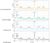 |
Fig. 20 X-ray diffraction spectra for the different material conditions: The figure presents the raw spectra with indexed austenite (γ) and martensite (α′) peaks. The four conditions are compared: (a) the as-received reference material, (b) the low-strain dome flange, (c) the medium-strain dome wall, and (d) the high-strain dome pole. |
Volume fractions of retained austenite and martensite determined by XRD.
5.7 Fatigue life of pre-formed membranes
The fatigue life of the manufactured membranes was evaluated experimentally. The tests were conducted on prototypes hydroformed at different pressures to investigate the influence of the forming process on the membrane durability. During the tests, the membrane was subjected to a cyclic pressure differential of 0.1 bar at an actuation frequency of 2 Hz. This pressure difference was generated by alternating the pressure on both sides of the membrane between 1.5 bar and 1.6 bar. The results are summarized in Table 4.
The results demonstrate a strong dependence of the fatigue life on the initial forming pressure and the resulting properties of the membrane (geometry, strains, residual stresses). The membrane formed at a pressure of 16 bar failed after 651,496 cycles. The fracture is shown in Figure 21.
In contrast, the membrane formed at the identified pressure of 14 bar exhibited an improved fatigue performance. The test for this membrane was stopped after 5,215,180 cycles without any signs of cracking or failure. This proves that the process window identified via simulation und experimentation results in a membrane with exceptional durability during operational performance.
For conventional flat metal diaphragms, the typical operational lifetime under ideal conditions is reported to be in the range of 3,000 to 5,000 h. This corresponds to approximately 64.8 to 108 million cycles at a typical operating frequency of 6 Hz, though this is often reduced by start-stop operation or non-ideal conditions [6].
Overview of the membrane fatigue limits after hydroforming at different pressures.
 |
Fig. 21 Failure mode of a hydroformed membrane after fatigue testing. The membrane was hydroformed with 16 bar. The fatigue crack is initiated in the dome wall, a region that possesses lower strain hardening from the forming process compared to the dome pole. An indentation zone is visible, proving non-axisymmetric behavior of the membrane. |
5.8 Realized increase in displaced volume
To determine the displaced volume under operational load (Tab. 4), the scanned membranes according to chapter 4.3 were used. It should be noted that the volume of the formed membranes was determined in clamped condition and only for deflection in forming direction under various operational pressures without a restricting cavity in the test rig, i.e., the volume of only one deflection mode (in forming direction) was evaluated experimentally to demonstrate the relative increase of displaced volume. The volume of the deflection in opposite direction to forming has not been determined experimentally. Thus, the total displaced volume for a complete stroke cannot be calculated. For testing of the fatigue life, dedicated cavities were used inside of the test rig influencing the deflection behavior of the membrane. Therefore, the volume of the cavity is also given in Table 4. As shown in Table 5, the hydroformed membrane (formed at 14 bar) provides a displaced volume of 39.2 cm3, which represents an increase of about 60% compared to the 24.6 cm3 of a conventional flat diaphragm of the same diameter and under the same operational pressure.
A further increase in displaced volume can be achieved by increasing the operational pressure. For a pressure value of 1 bar, the volume was increased by 94%. The effects of the increase of the pressure during operation on elastic deflection and fatigue life have not been tested yet. Additionally, the simulation of the deflection needs to be performed within dedicated cavities on both side to investigate the influence allowing to optimize the cavity geometry with regard to maximum displaced volume and maximum fatigue life.
Volume of the flat and deformed dome diaphragm with outer diameter of 140 mm.
6 Conclusion
This study demonstrated the significant improvement in the performance of a diaphragm compressor using pre-formed membranes made of spring-hard 1.4310 steel foil. A numerical and experimental methodology for the design, manufacturing and testing of pre-formed, bistable metal membranes for diaphragm compressors was developed and validated. By systematically investigating the entire process chain from material characterization and forming simulation to experimental prototyping and fatigue testing, the following key conclusions can be drawn:
A validated FE model was set up including elastic and plastic anisotropic material properties. The model was used to predict the membrane properties (e.g., geometry, strain and stress state, deflection behavior). The comparison between simulation and experiment resulted in maximum relative deviations of 21.3% which are related to material characterization, simplification of the model using plane symmetry and shell elements and assumptions of the chosen Hill48 yield criterion.
The membranes were manufactured by hydroforming in which the pressure is an important parameter. The optimal pressure for the hydroforming of the membrane was determined at 14 bar within the investigations. The hydroforming process in connection with the chosen tool design influences the geometry, strain and stress state of the membrane after springback. A non-homogeneous elastic and plastic strain distribution was observed. An optimal die cavity needs to be designed for the final target membrane geometry and for a more homogeneous strain distribution. In addition, the presence and effect of residual stresses have not been evaluated yet.
The key factors influencing the deflection behavior of the membrane are the final geometry and the resulting stiffness of the membarne along with the elastic and plastic properties of the material. The hardening behavior plays a crucial role with regard to the deflection of the membrane. For the 1.4310, a combined hardening due to work-hardening and the transformation of martensite. An XRD analysis provided a quantification of the TRIP effect, showing a systematic increase in martensite content from 17.3% in the as-received state to 30.4% at the dome pole with the highest plastic strains. The effect of deflection on the martensite content as well as the influence of martensite on the fatigue life (under hydrogen atmosphere) needs to be investigated.
A dome-shaped membrane geometry was developed and validated achieving an increase of the displaced volume of 60% at an operational pressure of 0.1 bar in comparison to the conventional flat diaphragm. The membrane formed at 14 bar endured over 5.2 million cycles without failure, proving its exceptional durability. The optimal design of the deflection cavity and the application of higher operational pressures need to be validated. A numerical simulation of the fatigue properties of the membrane would accelerate to development of improved designs.
Using pre-formed membranes in diaphragm compressors help to overcome the current limitation of conventional systems with flat membranes, where an increase in volume is typically associated with a drastic reduction in service life. In summary, this work provides an initial methodology for developing next-generation, high-performance diaphragms
Acknowledgments
The authors gratefully acknowledge the design, construction and initial set-up of the test rig for fatigue testing by Kyros Hydrogen Solutions GmbH and thank for their valuable support during the experimental testing phase of this work. The authors thank Dr. Florian Bittner from the Fraunhofer Institute for Machine Tools and Forming Technology (IWU) for conducting the X-ray diffraction measurements and for the explanation and discussion regarding the phase analysis. Furthermore, the authors thank Dr. Thomas Mehner from the Chair of Materials and Surface Engineering at the Chemnitz University of Technology for the quantitative evaluation of the phase fractions from XRD measurements.
Funding
The authors would like to thank the German Federal Ministry of Education and Research (Bundesministerium für Bildung und Forschung, BMBF) for funding the research project “PEM4heat - Entwicklung eines PEM Hochdruckelektrolyse Stacks mit Prozesswärmeauskopplung, eines H2-Hochdruckverdichters und eines Kreislaufmotors am WIR!-Ausgangspunkt Sonneberg”.
Conflicts of interest
The authors have nothing to disclose.
Data availability statement
No new data/codes were created or analyzed in this study.
Author contribution statement
Conceptualization, M.S., A.L. T.C., and V.K.; Methodology, M.S., A.L. and T.C.; FE simulation, M.S.; Experimental Validation, M.S.; Investigation and Analysis, M.S., M.P. and A.L.; Writing – Original Draft Preparation, M.S. and A.L.; Writing – Review & Editing, A.L., T.C. and V.K.; Visualization, M.S.; Supervision, V.K.; Project Administration, A.L..
References
- M. Balat, Potential importance of hydrogen as a future solution to environmental and transportation problems, Int. J. Hydrogen Energy, 33 (2008) 4013 [CrossRef] [Google Scholar]
- C.J. Winter, Hydrogen energy - abundant, efficient, clean: a debate over the energy-system-of-change, Int. J. Hydrogen Energy, 34 (2009) 1 [Google Scholar]
- J.E. Kang, T. Brown, W.W. Recker, G.S. Samuelsen, Refueling hydrogen fuel cell vehicles with 68 proposed refueling stations in California: Measuring deviations from daily travel patterns, Int. J. Hydrogen Energy, 39 (2014) 3444 [Google Scholar]
- K. Reddi, A. Elgowainy, E. Sutherland, Hydrogen refueling station compression and storage optimization with tube-trailer deliveries, Int. J. Hydrogen Energy, 39 (2014) 19169 [CrossRef] [Google Scholar]
- K. H. Küttner, Kolbenverdichter. In Kolbenmaschinen 170 (1984). https://doi.org/10.1007/978-3-663-10579-4_4 [Google Scholar]
- M. Dehnen, Hofer diaphragm compressors, 1998 [Google Scholar]
- https://www.sera-web.com/de/wasserstofftechnik/produkte/kompressoren/puseries (Updated: 20.10.2025) [Google Scholar]
- https://mehrer.de/de/produkte/membrankompressoren (Updated: 20.10.2025) [Google Scholar]
- W. Yu, X. Dianbo, F. Jianmei, P. Xueyuan, Research on sealing performance and self-acting valve reliability in high-pressure oil-free hydrogen compressors for hydrogen refueling stations, Int. J. Hydrogen Energy, 35 (2010) 8063 [Google Scholar]
- S. Ren, X. Jia, J. Zhang, X. Li, S. Zhang, X. Peng, Diagnosis method to identify diaphragm state of diaphragm compressors for hydrogen refueling stations based on dynamic oil pressure, Int. J. Hydrogen Energy, 49 (2024) 1043–1055 [Google Scholar]
- Y. Hu, X. Xu, W. Wang, A new cavity profile for a diaphragm compressor used in hydrogen fueling stations, Int. J. Hydrogen Energy, 42 (2017) 24458 [Google Scholar]
- J. Li, X. Jia, Z. Wu, X. Peng, The cavity profile of a diaphragm compressor for a hydrogen refueling station, Int. J. Hydrogen Energy, 39 (2014) 3926 [Google Scholar]
- X. Jia, J. Chen, H. Wu, X. Peng, Study on the diaphragm fracture in a diaphragm compressor for a hydrogen refueling station, Int. J. Hydrogen Energy, 41 (2016) 6412 [Google Scholar]
- B.A. Ivanov, S.E. Narkunskii, V.F. Pleshakov, N.I. Ul'yanov, Selection of materials for high pressure oxygen diaphragm compressors, Chem. Pet. Eng. 17 (1981) 306 [Google Scholar]
- P. Pavliuchenko, M. Teller, G. Hirt, Analysis of influencing factors on the achievability of bistable fully closed shells by semi-analytical modeling, ICTP, 13, 2319-2330, Cham: Springer International Publishing (2021) [Google Scholar]
- M. Solovev, A. Leonhardt, A. Graf, A. Kunke, V. Kräusel, Development of geometry variants and forming technology for metal diaphragms to increase the efficiency of diaphragm compressor, IOP Conf. Ser.: Mater. Sci. Eng. 1284 (2023) 1 [Google Scholar]
- M. Solovev, A. Leonhardt, A. Kunke, T. Clausmeyer, Increasing the displaced fluid volume of curved metal membranes for diaphragm compressors, MATEC Web Conf. 408 (2025). https://doi.org/10.1051/matecconf/202540801094 [Google Scholar]
- S. Friedrich, T. Mehner, A. Dittes, C. Binotsch, T. Clausmeyer, T. Lampke, B. Awiszus, Prediction of corrosion in the stainless steel 316L in the near-surface zone by numerical simulation, JOM, 77 (2025) 7529–7539 [Google Scholar]
- T. Wang, Z. Tang, X. Jia, Study on the stress and deformation of a diaphragm compressor cylinder head under extreme conditions, IOP Conf. Ser.: Mater. Sci. Eng. 604 (2019) 1 [Google Scholar]
- C. Zhang, Y. Lou, S. Zhang, T. Clausmeyer, A. E. Tekkaya, L. Fu, Q. Zhang, Large strain flow curve identification for sheet metals under complex stress states, Mech. Mat. 161 (2021). https://doi.org/10.1016/j.mechmat.2021.103997 [Google Scholar]
- S.K. Kang, Y.C. Kim, K.H. Kim, D. Kwon, J.Y. Kim, Constitutive equations optimized for determining strengths of metallic alloys, Mech. Mat. 73 (2014) 51 [Google Scholar]
- T.B. Mac, V.C. Do, D.T. Nguyen, A study of combined finite element method simulation/experiment to predict forming limit curves of steel DP350 sheets, Adv. Mech. Eng. 10 (2018). https://doi.org/10.1177/1687814018768148 [Google Scholar]
- Y. Yan, H. Wang, Q. Li, The inverse parameter identification of Hill 48 yield criterion and its verification in press bending and roll forming process simulations, J. Manuf. Process. 20 (2015) 46–53 [Google Scholar]
- J. Łuksza, M. Rumiński, W. Ratuszek, M. Blicharski, Texture evolution and variations of α-phase volume fraction in cold-rolled AISI 301 steel strip, J. Mater. Process. Technol. 177 (2006) 555 [Google Scholar]
Cite this article as: Mikhail Solovev, André Leonhardt, Murli Manohar Pandey, Verena Kräusel, Till Clausmeyer. Pre-formed metal membranes for diaphragm compressors: a combined numerical and experimental investigation of forming process and fatigue life, Manufacturing Rev. 13, 9 (2026), https://doi.org/10.1051/mfreview/2025029
All Tables
Overview of the membrane fatigue limits after hydroforming at different pressures.
All Figures
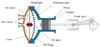 |
Fig. 1 Schematic of the operating principle of a single-stage diaphragm compressor [10]. |
| In the text | |
|
Fig. 2 Solution approach: Increase in stroke volume due to plastic deformation and hardening of the membrane: a) conventional, flat membrane (max. deflection under 0.1 bar –3.2 mm), b) pre-formed membrane (max. deflection under 0.1 bar –6.76 mm) and c) utilization of the hardening by forming. |
| In the text | |
|
Fig. 3 Experimentally determined (average) (a) and extrapolated (b) flow curves of the 1.4310 stainless steel foil. |
| In the text | |
|
Fig. 4 Position of samples taken from a hydroformed membrane (a) and the Bruker Discover D8 diffractometer used for quantifying phase fractions (b). |
| In the text | |
|
Fig. 5 Single-element model in Abaqus. |
| In the text | |
|
Fig. 6 FE model for the hydroforming process. The 3D quarter model shows the deformable blank (elasto-plastic), the rigid die, and the rigid blank holder. The active membrane radius is R = 70 mm. |
| In the text | |
|
Fig. 7 Target membrane dome geometry. |
| In the text | |
|
Fig. 8 Experimental setup for the hydroforming process: (a) the hydroforming tool set mounted in an electro-spindle press, showing the upper and lower die, (b) technical drawing of the cross-section of the upper die, detailing the dome-shaped tool cavity used for membrane manufacturing. |
| In the text | |
|
Fig. 9 Test rig for determining the fatigue limit of the pre-formed diaphragms during oscillating deflection. |
| In the text | |
|
Fig. 10 Pressure sensor signal for failure detection during fatigue testing. The plot shows the voltage output corresponding to the pressure level during cyclic deflection. The three signals before failure (left) show the characteristic progress of the bistable deflection. The signals after failure (right) indicate a clear and permanent drop in peak voltage, which was used as the criterion to determine the exact moment of fracture. |
| In the text | |
|
Fig. 11 The plots compare the predicted effective flow curves (dotted lines) in the 0° and 90° directions for the four different parametrization cases defined in Table 2: (a) A1, (b) A2, (c) B1, and (d) B2. The solid lines represent the original extrapolated input flow curves from experimental data. |
| In the text | |
|
Fig. 12 Validation of the FE model in comparison to the experimental geometry measurements: The cross-sectional profiles of the membrane after hydroforming and springback are compared. The plots show the results along the rolling direction (a) and the transverse direction (b). The anisotropic simulation (“Sim.”, black line) shows an improved prediction of the geometry in relation to the experimental data (“Exp.”, green line) in comparison with the simplified isotropic model (“Sim.*”, orange line). |
| In the text | |
|
Fig. 13 Comparison of membrane profiles along principal directions, showing the effect of anisotropy. The predicted (a) and experimentally measured (b) geometries are shown. In both cases, the final dome geometry differs depending on the direction, confirming the non-axisymmetric springback behavior. |
| In the text | |
|
Fig. 14 Comparison of simulated and experimental membrane profiles under operational load. The plots show the deflected cross-section of the membrane under a pressure of 0.1 bar, after the initial hydroforming and springback, (a) for Path A and (b) Path B. The anisotropic simulation (“Sim.”, black line) shows an improved prediction of the geometry in relation to the experimental data (“Exp.”, green line) in comparison with the simplified isotropic model (“Sim.*”, orange line). |
| In the text | |
|
Fig. 15 Influence of forming pressure on membrane geometry. Simulated membrane profiles at maximum forming pressure (a) and final predicted membrane profiles after unloading and springback, compared to the desired target geometry (b). |
| In the text | |
|
Fig. 16 Distribution of equivalent plastic strain (PEEQ) after springback for different forming pressures. The plots show the final PEEQ along Path A, evaluated at different section points through the membrane's thickness. (a) PEEQ at the top surface (opposite side of the die) and (b) PEEQ at the bottom surface (side of the die), revealing localized plastic deformation in the transition radius. |
| In the text | |
|
Fig. 17 Simulated membrane profiles during the second operational folding: (a) the plot shows the deflected shape of the hydroformed membranes under a 0.1 bar reverse pressure load; (b) the membranes formed at high pressures (> 16 bar, here 21 bar) fail to achieve a complete and stable reverse deflection. |
| In the text | |
|
Fig. 18 Evolution of strain components during hydroforming and springback. The plot on the left shows the strain state under the 14 bar forming load, composed of both plastic (PEEQ, PE22) and elastic (EE22) contributions (a). The plot on the right shows the final state after elastic recovery (b). |
| In the text | |
|
Fig. 19 Elastic deflection of the pre-formed membrane under operational load. The plots show the change in the membrane profile from the unloaded (sprung-back) state to the loaded state (0.1 bar). (a) FE simulation results. (b) Experimental measurements from the GOM system. |
| In the text | |
|
Fig. 20 X-ray diffraction spectra for the different material conditions: The figure presents the raw spectra with indexed austenite (γ) and martensite (α′) peaks. The four conditions are compared: (a) the as-received reference material, (b) the low-strain dome flange, (c) the medium-strain dome wall, and (d) the high-strain dome pole. |
| In the text | |
|
Fig. 21 Failure mode of a hydroformed membrane after fatigue testing. The membrane was hydroformed with 16 bar. The fatigue crack is initiated in the dome wall, a region that possesses lower strain hardening from the forming process compared to the dome pole. An indentation zone is visible, proving non-axisymmetric behavior of the membrane. |
| In the text | |
Current usage metrics show cumulative count of Article Views (full-text article views including HTML views, PDF and ePub downloads, according to the available data) and Abstracts Views on Vision4Press platform.
Data correspond to usage on the plateform after 2015. The current usage metrics is available 48-96 hours after online publication and is updated daily on week days.
Initial download of the metrics may take a while.